Norway and the Parabolic Fractal Law
Posted by Sam Foucher on July 6, 2006 - 12:51pm
URR= Ultimate Recoverable Ressource
PFL= Parabolic Fractal Law
HL= Hubbert Linearization
Mb= Millions of barrels
Gb= Billions of barrels
Norway's oil production is one of the most well documented production with complete data freely available on the Internet [10]. Production has been booming in the late 80s with a 50% growth in production between 1987 and 1992. However, production has peaked in 2001 and has declined dramatically afterward with a decline rate that mirrors the previous strong growth.
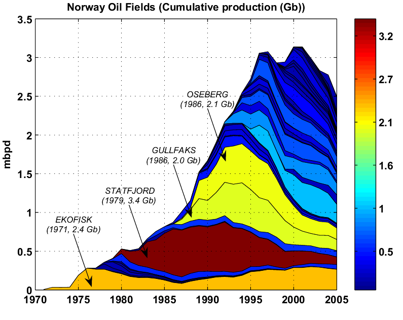
Fig. 1- Norway oilfields (crude oil only). GraphOilogy.
As we can see on Fig. 2, the Hubbert approach gives rather good results. The estimated URR is 26.54 Gb (crude oil only, no condensates) and the observed cumulative production is 19.2 Gb (72.5% of the URR).
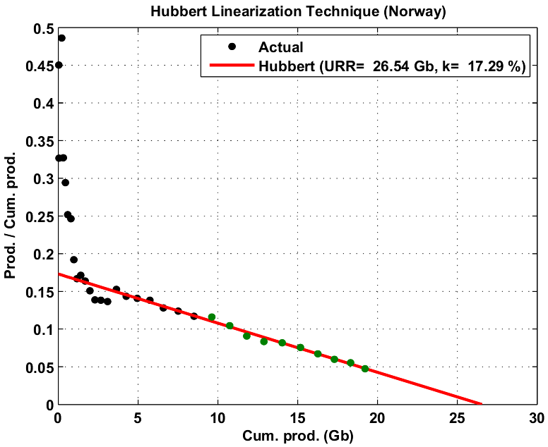
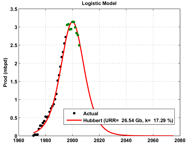
Fig. 2- Hubbert Linearization technique applied on
Norway Production
(green points are the data used for the fit).
We can appreciate how well the curve fitting is working for Norway by comparing with some reserve estimates given in Table I.
| Source | Year | Past Production (Gb) |
Reserve (Gb) | URR (Gb) |
|---|---|---|---|---|
| ASPO [7] | End 2001 | 15.2 |
16 | 31.2 |
| BP [9] | end 2005 |
19.2 |
9.7 | 28.9 |
| Oil & Gas Journal [8] | end 2005 |
19.2 | 7.7 | 26.9 |
| World Oil [8] | end 2004 |
14.0 |
9.86 | 25.0 |
Reserve estimates may include NGL.
The logistic growth rate (or decline rate) K for Norway is very large at 17% . One reason for that steep production growth and decline is maybe due to the very large decline rates observed on the top 5 fields as shown on Table II. Four of the top fields have values for K ranging from 25% to 37%! Fig. 3 gives the result of the logistic curve modeling on Statfjord which is at 98% of its URR. Only Ekofisk (Fig. 4), one of oldest field, can be seen as the remaining backbone of Norway's production with only a logistic decline rate at 8% and only 47% of its URR produced.
| Field | Q(2005) (Gb) | Starting Year | URR (Gb) | K (%) |
|---|---|---|---|---|
| Statfjord | 3.45 | 1979 |
3.53 | 25.8 |
| Ekofisk | 2.40 | 1971 |
5.10 | 8.3 |
| Oseberg | 2.12 | 1986 |
2.21 | 32.7 |
| Gullfaks | 2.04 | 1986 |
2.11 | 31.6 |
| Troll | 1.08 | 1990 |
1.43 | 36.8 |
URR and logistic growth (K) estimates using the HL technique.
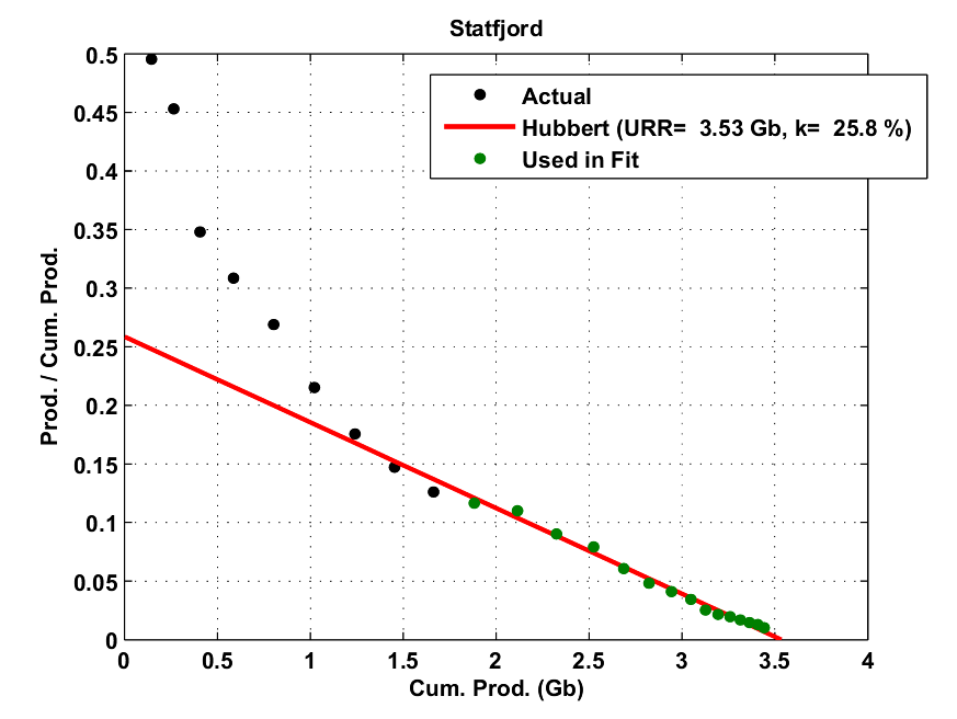
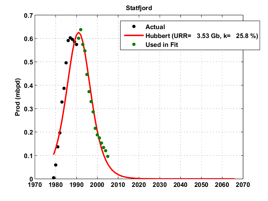
Fig. 3- HL technique applied on the Statfjord oilfield. The logistic curve peak position is computed
in order to have the same cumulative production in 2005.
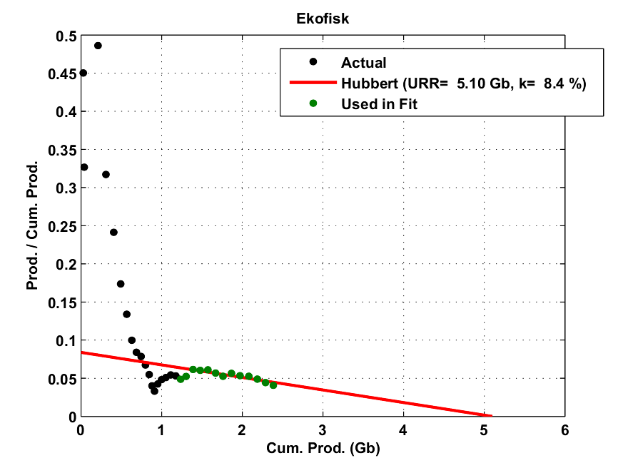
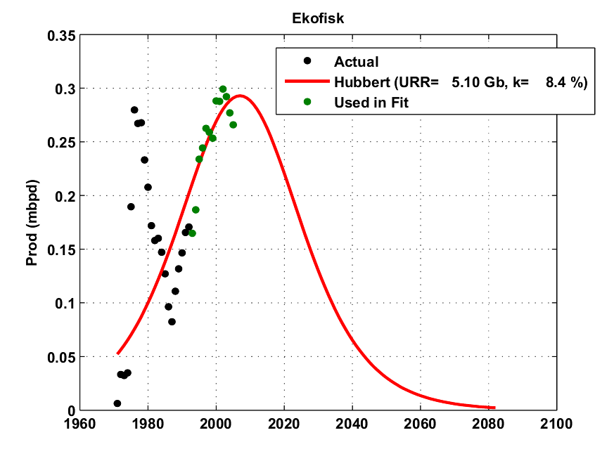
Fig. 4- HL technique applied on the Ekofisk oilfield. The logistic curve peak position is computed
in order to have the same cumulative production in 2005
The data for Norway contains production profiles for 47 oilfields. In order to get a more precise estimate of the PFL parameters, we perform the HL technique on each of the top 16 fields represented as empty circles on Fig. 5. Note that this refinement step does not change much the top of the PFL curve which is already very mature.
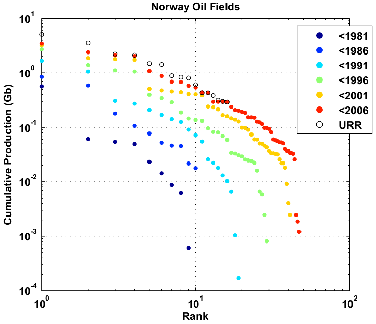
Fig. 5- Field cumulative production values displayed
in a log(size)-log(rank) plane at different points in time.
The empty circles are the URR estimates for the 16 top fields using the
HL technique.
The next step is to try to
fit a quadratic polynome using the
data representation shown on Fig. 6. Only the top 16 fields are used for the fit. The resulting
curvature is surprinsingly low at -0.31
which is more than four times the value obtain for the UK and the world
(-0.07) [2]. I
don't have a definitive answer on why this value is so low, one
possibility is the dataset contains too few oil fields (only 47). One
clue: In [5]
page 26, Jean Laherrère reports the following:
In UK only 52% of the discoveries are developed representing 89% of the reserves. In Norway, only 33% of the discoveries are developed representing 83% of the reserves.
Table III is from the same document and gives some details on the distribution of reserves for the UK and Norway (NW).
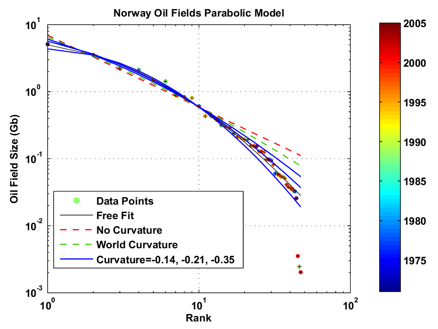
Fig. 6- Estimation of
various PF Laws with different
fixed curvature values.
Each data point is color coded according to the
oil field age..
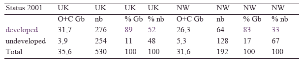
Table III. from Jean Laherrère [5], page 26: O= crude oil, C= Condensate, nb= number of fields.
Now, let's assume that we have a total number of fields around 200. This number will intersect the different Parabolic Fractal curves and is represented as an orange dotted line on Fig. 7. The intersection of this line with the different curves gives different URR and minimum size values as shown on Fig. 8. We can see that the world curvature (the orange disc) leads to an URR close to the ASPO and the official reserve numbers (the minimum field size is then around 7 Mb).
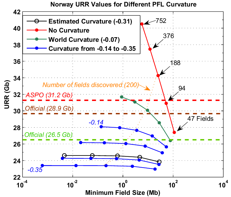
Fig. 7- Derived URR from
the PFL shown on Fig 6
for different curvature values and number of fields.
The orange dotted line is the isoline corresponding to 200 fields.
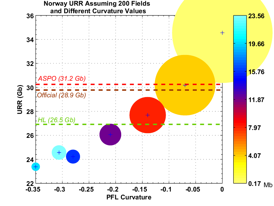
Fig. 8- Derived URR from Fig. 7 by fixing the number of fields
to 200 (dotted orange line on Fig. 8).
The disc size and color is function of the minimum field size.
HL is the URR estimate from the Hubbert Linearization shown on
Fig. 2.
Conclusion
- the Hubbert linearization gives an URR at 26.5 Gb
- the number of fields discovered is around 200
- the PFL + world curvature gives an URR between 26 and 32 Gb
- the PFL + world curvature + 200 fields gives an URR at 31 Gb
References
[1] TOD: An Attempt to Apply The Parabolic Fractal Law to Saudi Arabia[2] GraphOilogy: What Can We Learn From The Oil Field Size Distribution?
[3] GraphOilogy: Some Detailed Views on Norway's Oil Production
[4] Jean Laherrère: “Parabolic fractal” distributions in Nature. (in French)
[5] Jean Laherrère: Estimates of Oil Reserves
[6] ASPO: Newsletter 62 (2006/02)
[7] ASPO: Newsletter 25 (2003/01)
[8] World Proved Reserves of Oil and Natural Gas, Most Recent Estimates
[9] BP: Statistical Review of World Energy 2006
[10] Norwegian Petroleum Directorate
Contact
- Content: editors at theoildrum dot com
- Tech support: support at theoildrum dot com
License

This work is licensed under a Creative Commons Attribution-Share Alike 3.0 United States License.
I imagine you must know Stuart and one point I have made to him in recent days is that the really important thing to understand is what is going on inside ME- OPEC - I can already hear the regular TODers groaning in dismay - what has been known to a few for a long time, however, is news to a FNG.
My understanding of the Saudi field development history, by way of example, is that only the super giants have been fully developed - Ghawar, Abqaiq, Berri, Safaniya and Shaybah. The rest it seems has been largely ignored - what was the point in developing everything else when you had to keep you super giants choked back for decades?
What I was wondering was what Norway's production profile would look like if they only produced Ekofisk, Statfjord, Oseberg, Gullfaks ± Troll, ± Snorre until these fields peaked. You then panic and decide to produce everything else - and this may produce a second peak on the down curve from the biguns. Just an idea that may give a clue how the Saudi (Kuwait and UAE) production profiles may pan out over the next 20 years.
Your charts and work on Norway are fantastic.
HL big fields:
HL small fields:
Clearly production have been maintained by the 42 smallest fields that contains 50% of the URR. The contribution from the top 5 has peaked in 1995 whereas the small fields contribution has peaked in 2002. I'm surprised that the decline rates are similar (~22%).
Very interesting to see that the 42 smallest fields reach a peak that is just marginally higher than the 5 biggest. This I think is a good thing. If KSA do indeed have 42± smaller fields to develop (in their size scale) then is it possible that KSA may have a second peak in 25 years time?
There's no doubt that KSA will have a large number of undeveloped fields - p 33 of Twilight shows some of these. It will require a huge amount of cash and effort to develop them. This may have no impact on peak oil but may have a profound impact on the shape of the down curve.
PS its 11 o'clock here in Aberdeen and I'm off trout fishing in Norway tomorrow and am not back till Tuesday.
I just continue to be baffled by the numbers coming out of these posts. Besides of the mystic 0.07, now that equal K for the big and smaller fields.
The equal K must be a symptom of a fractal phenomenon. The smaller fields behave just like the big ones!
Had we field by field data for KSA, we could get a pretty good idea of what the production of smaller fields will look like.
All in all I think KSA will yield a future production graph over time like that of the UK, with a primary peak followed by a second. In the UK this was due to two separate discovery cycles; in KSA this will be due to two development cycles.
The result - KSA peaked in 1980 and that's it.
Why not?
See my comments on figuring telescope mirrors elsewhere.
OTOH, consider that in 1999 SA chose to devlop Shaybah, located very deep in the empty quarter, where production costs are much higher, and anyway development required expensive, horizontal multilateral wells. Presumably, this was at that time their lowest cost option.
BTW, their doubling of rigs may be necessary to maintain production because they are now resorting to horizontal wells, which take longer to drill.
The post-1970 cumulative Lower 48 production was 99% of what the HL model predicted that it would be. What is interesting is that unrestrained drilling for smaller fields had no discernible effect.
If you use only cumulative production you will get a log-normal distribution unless the producing region is very mature. As production mature, the parabola curvature should tends toward zero i.e. a straight line which represents perfect self-similarity. The idea is to try to fit the parabola only on the top fields which are genrally the most mature as it is the case for Norway, UK and Saudi Arabia. Notice in Fig. 5, how the shape formed by the top fields is quite stable. The smaller fields are usually less mature and will depart strongly from the parabolic fractal hence the log-normal shape. The idea is to use only the top fields to estimate the PFL parameters. A quote from Laherrere:
src
Agreed. There are no theoretical justifications in adding a quadratic term. It`s an heuristic model proposed by Laherrere that produced quite good results on city and galaxy size distributions. For instance, you can estimate the US population from the size distribution of the top 257 US urban agglomerations (188 millions of people):(Minh= millions of people)
I don't think it is more accurate but it may provide us with an orthogonal way to estimate a URR range. It may help clarify difficult cases such as Saudi Arabia. Note that the HL on SA is points toward 180 Gb for the URR whereas conservative sources such as the ASPO are saying 260 Gb. The HL technique is interesting for unconstraint production profiles where cumulative production is near 50% of the URR.
In the polarised argument about Saudi, OPEC and World reserves I beleive both sides may be right.
Does KSA have vast undeveloped reserves? The answer is probably yes - analogous to the 42 smaller Norwegian Fields. In KSA some of these will have been developed and switched on and off over the years - but what was the point developing them when you have one field doing 5 million bopd - and it was choked back.
Is KSA production about to crater, Simmons style? The answer is probably yes because development work on "all the rest" has started too late.
Where I believe the Saudis may be in denial is accepting that production from the 5 super giants is going to go into sharp decline. They would like to project current production out into the future and add new developments on to this - giving rise to production estimates of 15 million bopd etc. Infact what is more likely to happen, is that production will fall sharply near term but may build again in 10 to 20 years time if they are able to efficiently develop "all the rest."
What the Saudis may be doing now by way of developing smaller fields will come too late to impact world peak which I think is fast approaching - if recent price beahaviour is any guide. What is important to bear in mind is that peak itself may not be that important. It is demand rising faster than production growth that will drive up prices and cause fuel shortages, initially in the poorer countries.
Is the world economy stuffed? Probably yes.
Most of the country by area, I would suggest, is proportionately no richer in oil than most of the US, for example. Saudi Arabia overall has proportionately much more oil because in the lone Eastern Province there are the world's biggest fields, whereas in Texas or Alaska there are just very big ones.