Application of the Dispersive Discovery Model
Posted by Sam Foucher on November 27, 2007 - 11:00am
This is a guest post by WebHubbleTelescope.
Sometimes I get a bit freaked out by the ferocity and doggedness of the so-called global warming deniers. The latest outpost for these contrarians, climateaudit.org, shows lots of activity, with much gnashing over numbers and statistics, with the end result that they get a science blog of the year award (a 1st place tie actually). Fortunately, the blog remains open to commenting from both sides of the GW argument, which if nothing else makes it a worthy candidate for some type of award. Even though I don't agree with the nitpicking approach of the auditors, they do provide peer review for strengthening one's arguments and theories. I can only hope that this post on oil depletion modeling attracts the same ferocity from the peak oil deniers out there. Unfortunately, we don't have a complementary "oil depletion audit" site organized yet (though Stuart and Khebab, et al, seem to be working on it--see yesterday's post), so we have to rely on the devil's advocates on TOD to attempt to rip my Application of the Dispersive Discovery Model to shreds. Not required, but see my previous post Finding Needles in a Haystack to prime your pump.
 |
A Premise In Regards To The Pyramid
I start with one potentially contentious statement: roughly summarized
as "big oil reserves are NOT necessarily found first".
I find this rather important in terms of the recent work that Khebab and Stuart
have posted. As Khebab notes "almost half of the
world production is coming from less than 3% of the total number of
oilfields". So the intriguing notion remains, when
do these big oil finds occur, and can our rather limited understanding
of the discovery dynamics provide the Black Swan moment1 that the PO denialists
hope for? For a moment, putting on the hat of a denier, one
could argue that we have no knowledge as to whether we have found all
the super-giants, and that a number of these potentially remain,
silently lurking in the shadows and just waiting to get discovered.
From the looks of it, the USGS has some statistical confidence that
these exist and can make a substantial contribution to future reserves.
Khebab has done interesting work in duplicating the USGS results
with the potential for large outliers -- occurring primarily from the
large variance in field sizes provided by the log-normal field size distribution
empirically observed.
But this goes against some of the arguments I have seen on TOD
which revolve around some intuitive notions and conventional wisdom of
always finding big things first. Much like the impossibility of
ignoring the elephant in the room, the logical person would infer that
of course we would find big things first. This argument has
perhaps tangential scientific principles behind it, mainly in
mathematical strategies for dealing with what physicists call
scattering cross-sections and the like. Scientifically based or not, I
think people basically latch on to this idea without much thought.
But I have still have problems with the conventional
contention, primarily in understanding what would cause us to uniformly
find big oil fields first. On the one hand, and in historic terms,
early oil prospectors had no way of seeing everything under the earth;
after all, you can only discover what you can see (another bit of
conventional wisdom). So this would imply as we probe deeper
and cast a wider net, we still have a significant chance of discovering
large oil deposits. After all, the mantle of the earth remains a rather
large volume.
On the the same hand, the data does not convincingly back up
the early discovery model. Khebab's comment section noted the work of Robelius.
Mr. Robelius dedicated graduate thesis work to tabulating the portion
of discoveries due to super-giants and it does in fact appear to skew
to earlier years than the overall discovery data. However, nothing
about the numbers of giant oil fields
found appears skewed about the peak as shown in Figure 2
below:

Figure 2: Robelius data w/ASPO total superimposed
 |
| Figure 3: Discovery data of unknown origins |
 |
As is typical of discovery data, I do spot some
inconsistencies in the chart as well. I superimposed a chart provide by Gail of total discoveries due to ASPO
on top of the Robelius data and it appears we have an inversion or two
(giants > total in the 1920's and 1930's). Another graph from
unknown origins (Figure 3) has the same 62% number
that Robelius quotes for big oil contribution. Note that the number of
giants before 1930 probably all gets lumped at 1930. It still
looks inconclusive whether a substantial number of giants occurred
earlier or whether we can attach any statistical significance to the
distribution.
The controversial "BOE" discovery data provided by Shell
offers up other supporting evidence for a more uniform distribution of
big finds. As one can see in Figure 4 due to some
clearly marked big discoveries in the spikes at 1970 and 1990, the
overall discovery ordering looks a bit more stationary.
Unfortunately, I have a feeling that the big finds marked come about
from unconventional sources. Thus, you begin to understand the
more-or-less truthful BOE="barrel of oil equivalent" in small lettering
on the y-axis (wink, wink). And I really don't understand what their
"Stochastic simulation" amounts to -- a simple moving average perhaps?
--- Shell Oil apparently doesn't have to disclose their methods (wink,
wink, wink).
Given the rather inconclusive evidence, I contend that I can
make a good conservative assumption that the size of discoveries
remains a stationary property of any oil discovery model. This has some
benefits in that the conservative nature will suppress the pessimistic
range of predictions, leading to a best-case estimate for the
future. Cornucopians say that we will still find big
reservoirs of oil somewhere. Pessimists say that historically we have
always found the big ones early.
In general, the premise assumes no bias in terms of when we
find big oil, in other words we have equal probability of finding a big
one at any one time.
Two Peas to the Pod
For my model of oil depletion I intentionally separate the Discovery
Model from the Production Model. This differs from the
unitarians who claim that a single equation, albeit a heuristic one
such as the Logistic, can effectively model the dynamics of
oil depletion. From my point-of-view, the discovery process remains
orthogonal to the subsequent extraction/production process, and that
the discovery dynamics acts as a completely independent stimulus to
drive the production model. I contend that the two convolved
together give us a complete picture of the global oil depletion process.
 |
As for the Production Model, I continue to stand by the Oil Shock Model as a valid pairing to the Dispersive Discovery model. The Shock Model will take as a forcing function basically any discovery data, including real data or, more importantly, a model of discovery. The latter allows us to make the critical step in using the Shock Model for predictive purposes. Without the extrapolated discovery data that a model will provide, the Shock Model peters out with an abrupt end to forcing data, which usually ends up at present time (with no reserve growth factor included).
As for the main premise behind the Shock Model, think in terms
of rates acting on volumes of found material. To 1st-order,
the depletion of a valuable commodity scales proportionately to the
amount of that commodity on hand. Because of the stages that oil goes
through as it starts from a fallow, just-discovered reservoir, one can
apply the Markov-rate law through each of the stages. The Oil
Shock Model essential acts as a 4th-order low
pass filter and removes much of the fluctuations introduced by a noisy
discovery process (see next section). The "Shock" portion
comes about from perturbations applied to the last stage of extraction,
which we can use to model instantaneous socio-political
events. I know the basic idea behind the Oil Shock Model has
at least some ancestry; take a look at "compartmental models" for
similar concepts, although I don't think anyone has seriously applied
it to fossil fuel production and nothing yet AFAIK in terms of the
"shock" portion (Khebab has since applied it to a hybrid model).
Dispersive Discovery and Noise
 |
The shape of the curve that Jerry found due to Hubbert has the characteristic of a cumulative dispersive swept region in which we remove the time dependent growth term, retaining the strictly linear mapping needed for the histogram, see the n=1 term in Figure 7 below:
Figure 7: Order n=1 gives the cumulative swept volume mapped linearly to time
For the solution, we get:
wheredD/dh = c * (1-exp(-k/h)*(1+k/h))
h denotes the cumulative depth.I did a quickie overlay with a scaled dispersive profile, which shows the same general shape (Figure 8).
Figure 8: Hubbert data mapping delta discoveries to cumulative drilled footage
The
k term has significance in terms of an
effective URR as I described in the dispersive
discovery model post. I eyeballed the scaling as k=0.7e9 and c=250, so I
get 175 instead of the 172 that Hubbert got.To expand in a bit more detail, the basic parts of the derivation that we can substantiate involve the L-bar calculation in the equations in Figure 9 below (originally from):

Figure 9: Derivation of the Dispersed Discovery Model
The key terms include lambda, which indicates cumulative footage, and the L-bar, which denotes an average cross-section for discovery for that particular cumulative footage. This represents Stage-1 of the calculation -- which I never verified with data before -- while the last lines labeled "Linear Growth" and "Parabolic Growth" provide examples of modeling the Stage-2 temporal evolution.
Since the results come out naturally in terms of cumulative discovery, it helps to integrate Hubbert's yearly discovery curves. So Figure 10 below shows the cumulative fit paired with the yearly (the former is an integral of the latter):
 |
 |
I did a least-squares fit to the curve that I eyeballed initially and the discovery asymptote increased from my estimated 175 to 177. I've found that generally accepted values for this USA discovery URR ranges up to 195 billion barrels in the 30 years since Hubbert published this data. This, in my opinion, indicates that the model has potential for good predictive power.
 |
 |
 |
Although a bit unwieldy, one can linearize the dispersive discovery curves, similar to what the TOD oil analysts do with Hubbert Linearization. In Figure 13, although it swings wildly initially, I can easily see the linear agreement, with a correlation coefficient very nearly one and a near zero extrapolated y-intercept. (note that the naive exponential that Hubbert used in Figure 11 for NG overshoots the fit to better match the asymptote but still falls short of the alternative model's asymptote, and which also fits the bulk of the data points much better)
 |
 |
Every bit of data tends to corroborate that the dispersive discovery model works quite effectively in both providing an understanding on how we actually make discoveries in a reserve growth fashion and in mathematically describing the real data.
So at a subjective level, you can see that the cumulative ultimately shows the model's strengths, both from the perspective of the generally good fit for a 2-parameter model (asymptotic value + cross section efficiency of discovery), but also in terms of the creeping reserve growth which does not flatten out as quickly as the exponential does. This slow apparent reserve growth matches empirical-reality remarkably well. In contrast, the quality of Hubbert's exponential fit appears way off when plotted in the cumulative discovery profile, only crossing at a few points and reaching an asymptote well before the dispersive model does.
But what also intrigued me is the origin of noise in the discovery data and how the effects of super fields would affect the model. You can see the noise in the cumulative plots from Hubbert above (see Figures 6 & 11 even though these also have a heavy histogram filter applied) and also particularly in the discovery charts from Laherrere in Figure 14 below.

Figure 14: Unfiltered discovery data from Laherrere
If you consider that the number of significant oil discoveries runs in the thousands according to The Pyramid (Figure 1), you would think that noise would abate substantially and the law of large numbers would start to take over. Alas, that does not happen and large fluctuations persist, primarily because of the large variance characteristic of a log-normal size distribution. See Khebab's post for some extra insight into how to apply the log-normal, and also for what I see as a fatal flaw in the USGS interpretation that the log-normal distribution necessarily leads to a huge uncertainty in cumulative discovery in the end. From everything I have experimented with, the fluctuations do average out in the cumulative sense, if you have a dispersive model underlying the analysis, of which the USGS unfortunately leave out.
The following pseudo-code maps out the Monte Carlo algorithm I
used to generate statistics (this uses the standard trick for
inverting
an exponential distribution and a more detailed one for
inverting the Erf() which results from the
cumulative Log-Normal distribution). This algorithm draws on
the initial premise that fluctuations in discovering is basically a
stationary process, and remains the same over the duration of
discovery.
 |
Basic algorithmic steps:1 for Count in 1..Num_Paths loop
Lambda (Count) := -Log (Rand);
end loop;
2 while H < Depth loop
H := H + 1.0;
Discovered := 0;
3 for Count in 1 .. Num_Paths loop
4 if H * Lambda(Count) < L0 then
5 LogN := exp(Sigma*Inv(Rand))/exp(Sigma*Sigma/2.0);
6 Discovered := Discovered + Lambda(Count) * LogN;
end if;
end loop;
7 -- Print H + Discovered/Depth or Cumulative Discoveries
end loop;
- Generate a dispersed set of paths that consist of random lengths normalized to a unitary mean.
- Start increasing the mean depth until we reach some
artificial experimental limit (much larger than L0).
- Sample each path within the set.
- Check if the scaled dispersed depth is less than the estimated maximum depth or volume for reservoirs, L0.
- Generate a log-normal size proportional to the
dimensionless dispersive variable Lambda
- Accumulate the discoveries per depth
- If you want to accumulate over all depths, you will get
something that looks like Figure 15.
The series of MC experiments in Figures 16-22 apply various size sampling distributions to the Dispersive Discovery Monte Carlo algorithm4. For both a uniform size distribution and exponential damped size distribution, the noise remains small for sample sets of 10,000 dispersive paths. However, by adding a log-normal size distribution with a large variance (log-sigma=3), the severe fluctuations become apparent for both the cumulative depth dynamics and particularly for the yearly discovery dynamics. This, I think, really explains why Laherrere and other oil-depletion analysts like to put the running average on the discovery profiles. I say, leave the noise in there, as i contend that it tells us a lot about the statistics of discovery.
Figure 16: Dispersive Discovery Model mapped into Hubbert-style cumulative efficiency. The Monte Carlo simulation in this case is only used to verify the closed-form solution as a uniform size distribution adds the minimal amount of noise, which is sample size limited only.
Figure 17: Dispersive Discovery Model with Log-Normal size distribution. This shows increased noise for the same sample size of N=10000.
Figure 18: Same as Fig. 17, using a different random number seed
Figure 19: Dispersive Discovery Model assuming uniform size distribution
Figure 20: Dispersive Discovery Model assuming log-normal size distribution
Figure 21: Dispersive Discovery Model assuming log-normal size distribution. Note that sample path size increased by a factor of 100 from Figure 20. This reduces the fluctuation noise considerably.
Figure 22: Dispersive Discovery Model assuming exponentially damped size distribution. The exponential has a much narrower variance than the log-normal.
I figure instead of filtering the data via moving averages, it might make more sense to combine discovery data from different sources and use that as a noise reduction/averaging technique. Ideally I would also like to use a cumulative but that suffers a bit from not having any pre-1900 discovery data.
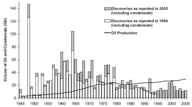
Figure 23: Discovery Data plotted with minimal filtering

Figure 24: Discovery Data with a 3-year moving average
Application of the Dispersive
Discovery + Oil Shock Model to Global Production
In Figure 2, I overlaid a Dispersive Discovery fit to the data. In this section of the post, I explain the rational for the parameter selection and point out a flaw in my original assumption when I first tried to fit the Oil Shock Model a couple of years ago.
Jean Laherrere of ASPO France last year presented a paper entitled "Uncertainty on data and forecasts". A TOD commenter had pointed out the following figures from Pp.58 and 59:
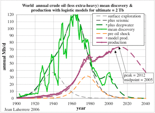
Figure 25: World Crude Discovery Data
Figure 26: World Crude Discovery Data
I eventually put two and two together and realized that the NGL portion of the data really had little to do with typical crude oil discoveries; as finding oil only occasionally coincides with natural gas discoveries. Khebab has duly noted this as he always references the Shock Oil model with the caption "Crude Oil + NGL". Taking the hint, I refit the shock model to better represent the lower peak of crude-only production data. This essentially scales back the peak by about 10% as shown in the second figure above. I claim a mixture of ignorance and sloppy thinking for overlooking this rather clear error.
So I restarted with the assumption that the discoveries comprised only crude oil, and any NGL would come from separate natural gas discoveries. This meant that that I could use the same discovery model on discovery data, but needed to reduce the overcompensation on extraction rate to remove the "phantom" NGL production that crept into the oil shock production profile. This essentially will defer the peak because of the decreased extractive force on the discovered reserves.
I fit the discovery plot by Laherrere to the dispersive discovery model with a cumulative limit of 2800 GB and a cubic-quadratic rate of 0.01 (i.e n=6 for the power-law). This gives the blue line in Figure 27 below.
Figure 27: Discovery Data + Shock Model for World Crude
For the oil shock production model, I used {fallow,construction,maturation} rates of {0.167,0.125,0.1} to establish the stochastic latency between discovery and production. I tuned to match the shocks via the following extraction rate profile:
Figure 28: Shock profile associated with Fig.27
As a bottom-line, this estimate fits in between the original oil shock profile that I produced a couple of years ago and the more recent oil shock model that used a model of the perhaps more optimistic Shell discovery data from earlier this year. I now have confidence that the discovery data by Shell, which Khebab had crucially observed had the cryptic small print scale "boe" (i.e. barrels of oil equivalent), should probably better represent the total Crude Oil + NGL production profile. Thus, we have the following set of models that I alternately take blame for (the original mismatched model) and now dare to take credit for (the latter two).
Original Model(peak=2003)
< No NGL(peak=2008)
< Shell data of BOE(peak=2010)
I still find it endlessly fascinating how the peak position of the models do not show the huge sensitivity to changes that one would expect with the large differences in the underlying URR. When it comes down to it, shifts of a few years don't mean much in the greater scheme of things. However, how we conserve and transition on the backside will make all the difference in the world.
Production as Discovery?
In the comments section to the dispersive oil discovery model post, Khebab applied the equation to USA data. As the model should scale from global down to distinct regions, these kinds of analyses provide a good test to the validity of the model.
In particular, Khebab concentrated on the data near the peak position to ostensibly try to figure out the potential effects of reserve growth on reported discoveries. He generated a very interesting preliminary result which deserves careful consideration (if Khebab does not pursue this further, I definitely will). In any case, it definitely got me going to investigate data from some fresh perspectives. For one, I believe that the Dispersive Discovery model will prove useful for understanding reserve growth on individual reservoirs, as the uncertainty in explored volume plays in much the same way as it does on a larger scale. In fact I originally proposed a dispersion analysis on a much smaller scale (calling it Apparent Reserve Growth) before I applied it to USA and global discoveries.
As another example, after grinding away for awhile on the available USA production and discovery data, I noticed that over the larger range of USA discoveries, i.e. inferring from production back to 1859, the general profile for yearly discoveries would not affect the production profile that much on a semi-log plot. The shock model extraction model to first order shifts the discovery curve and broadens/scales the peak shape a bit -- something fairly well understood if you consider that the shock model acts like a phase-shifting IIR filter. So on a whim, and figuring that we may have a good empirical result, I tried fitting the USA production data to the dispersive discovery model, bypassing the shock model response.
I used the USA production data from EIA which extends back to 1859 and to the first recorded production out of Titusville, PA of 2000 barrels (see for historical time-line). I plotted this in Figure 29 on a semi-log plot to cover the substantial dynamic range in the data.

Figure 29: USA Production mapped as a pure Discovery Model
This curve used the n=6 equation, an initial t_0 of 1838, a value for k of 0.0000215 (in units of 1000 barrels to match EIA), and a Dd of 260 GB.
D(t) = kt6*(1-exp(-Dd/kt6))The peak appears right around 1971. I essentially set P(t) = dD(t)/dt as the model curve.
dD(t)/dt = 6kt5*(1-exp(-Dd/kt6)*(1+Dd/kt6))
 |
Stuart Staniford of TOD originally tried to fit the USA curve on a semi-log plot, and had some arguable success with a Gaussian fit. Over the dynamic range, it fit much better than a logistic, but unfortunately did not nail the peak position and didn't appear to predict future production. The gaussian also did not make much sense apart from some hand-wavy central limit theorem considerations.
Even before Staniford, King Hubbert gave the semi-log fit a try and perhaps mistakenly saw an exponential increase in production from a portion of the curve -- something that I would consider a coincidental flat part in the power-law growth curve.
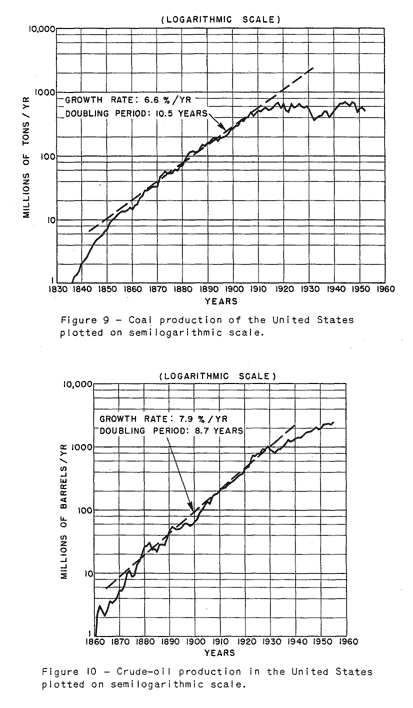
Figure 31: World Crude Discovery Data
Conclusions
The Dispersive Discovery model shows promise at describing:- Oil and NG discoveries as a function of cumulative depth.
- Oil discoveries as a function of time through a power-law
growth term.
- Together with a Log-Normal size distribution, the
statistical fluctuations in discoveries. We can easily represent the
closed-form solution in terms of a Monte Carlo algorithm.
- Together with the Oil Shock Model, global crude oil production.
- Over a wide dynamic range, the overall production shape.
Look at USA production in historical terms for a good example.
- Reserve growth of individual reservoirs.
References
1 "The Black Swan: The Impact of the Highly Improbable" by Nassim Nicholas Taleb. The discovery of a black swan occurred in Australia, which no one had really explored up to that point. The idea that huge numbers of large oil reservoirs could still get discovered presents an optical illusion of sorts. The unlikely possibility of a huge new find hasn't as much to do with intuition, as to do with the fact that we have probed much of the potential volume. And the maximum number number of finds occur at the peak of the dispersively swept volume. So the possibility of finding a Black Swan becomes more and more remote after we explore everything on earth.
2 These same charts show up in an obscure Fishing Facts article dated 1976, where the magazine's editor decided to adapt the figures from a Senate committee hearing that Hubbert was invited to testify to.
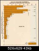
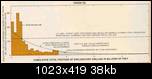
Fig. 5 Average discoveries of crude oil per loot lor each 100 million feet of exploratory drilling in the U.S. 48 states and adjacent continental shelves. Adapted by Howard L. Baumann of Fishing Facts Magazine from Hubbert 1971 report to U.S. Senate Committee. "U.S. Energy Resources, A Review As Of 1972." Part I, A Background Paper prepared at the request of Henry M. Jackson, Chairman: Committee on Interior and Insular Affairs, United States Senate, June 1974.Like I said, this stuff is within arm's reach and has been, in fact, staring at us in the face for years.
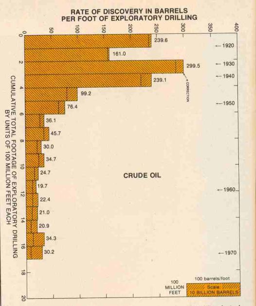
Fig.6 Estimation of ultimate total crude oil production for the U.S. 48 states and adjacent continental shelves; by comparing actual discovery rates of crude oil per foot of exploratory drilling against the cumulative total footage of exploratory drilling. A comparison is also shown with the U.S. Geol. Survey (Zapp Hypothesis) estimate.

3 I found a few references which said "The United States has proved gas reserves estimated (as of January 2005) at about 192 trillion cubic feet (tcf)" and from NETL this:
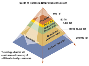 U.S. natural gas produced to date (990 Tcf) and proved reserves currently being targeted by producers (183 Tcf) are just the tip of resources in place. Vast technically recoverable resources exist -- estimated at 1,400 trillion cubic feet -- yet most are currently too expensive to produce. This category includes deep gas, tight gas in low permeability sandstone formations, coal bed natural gas, and gas shales. In addition, methane hydrates represent enormous future potential, estimated at 200,000 trillion cubic feet.This together with the following reference indicate the current estimate of NG reserves lies between 1173 and 1190 TCF (Terra Cubic Foot = 1012 ft3).
How much Natural Gas is there? Depletion Risk and Supply Security Modelling
US NG Technically Recoverable Resources US NG Resources
(EIA, 1/1/2000, Trillion ft3) (NPC, 1/1/1999, Trillion ft3)
--------------------------------------- -----------------------------
Non associated undiscovered gas 247.71 Old fields 305
Inferred reserves 232.70 New fields 847
Unconventional gas recovery 369.59 Unconventional 428
Associated-dissolved gas 140.89
Alaskan gas 32.32 Alaskan gas (old fields) 32
Proved reserves 167.41 Proved reserves 167
Total Natural Gas 1190.62 Total Natural Gas 1779
4 I have an alternative MC algorithm here that takes a different approach and shortcuts a step.
Contact
- Content: editors at theoildrum dot com
- Tech support: support at theoildrum dot com
License

This work is licensed under a Creative Commons Attribution-Share Alike 3.0 United States License.
http://science.reddit.com/info/61jei/comments/
thanks for your support.
Maths vs Politics
I'll repeat a statement made a few times before. If you want to use maths to predict/understand oil production/discoveries etc. then you need to explicitly 'reverse out' the impact of political and economic decisions.
Its no good trying to model areas such as new discoveries if you haven't taken into account the times when countries and oil companies "couldn't be bothered" to search exhaustively since they already had more reserves than they knew what to do with.
Equally if there is a recession and share price is troubled, oil companies will reduce the cost base and limit their exploration.
And then there are the technology shocks which introduce step changes into the system.
Trying to match maths to this noisy data with all these effects still in place artificially limits what you can understand. We KNOW when the recessions were, when the shocks occurred, etc. - so its possible to make allowance for them. Model on the cleaned up data, then add back in the real world effects and you can generate a tool that you can use to predict the 'perfect' world performance, and then add in your expected or observed real world events as they happen - essentially playing 'what if' scenarios.
Frankly, I look a little askew at a model that claims to accurately model the real world data without the taking account of the real world noise. It doesn't pass the sniff test.
Is it really that important?
We are talking an approximation here.
Let's assume the real world shocks are roughly evenly spread out in time, then the noise stays there, but does not affect the overall conclusion that much.
Also, whether the shocks have a relative big enough scale to matter, remains to me at least unproven.
I think the model has a lot of potential and cleaning the real world data would also have it's consequences, just as WHT points out. There have already been other methods using various ways of trying to average out the noise, perhaps introducing additional skew to the data for future extrapolation.
Modelling it with noise intact at least starts with a different premise and the results are encouraging.
However, in an ideal scenario, I think your point about trying to achieve 'perfect world' scenario is a good one.
BTW, great work WHT. Even a person like me who's getting back to physics/maths after at 15+ hiatus could follow the main gist of the article much of the time. That is quite remarkable communication and explanation powers you have!
Well, if you take the global oil production curve and work out the offsets, translations and stretching necessary to turn that shape into a smooth bell curve unconstrained consumption theory predicts - you can readily see how the effects I describe can have a key impact on production data. Its not a big step to suggest the effect is equivalent or greater in other areas.
So yes, I'd say its important.
Your points may have validity which might be checked by doing a sensitivity analysis, but one needs to start with a model, and the simplier the better. With a model in hand, one can introduce factors as you mention, and see how the model results deviate from the data. You can't reject the model as insignificant when you don't know how it responds to the input you suggest.
My suggestion is rather the reverse.
Take out of the base data the effect of known factors, then model the now simpler data. No mathematical equation will match the discontinuous actions of politics and economics - but take them out and you have a chance.
Once you have the model, add the effects back in.
I understand your point. The step changes I think are very deterministic and happen at the last stage of the process, which is why I call them shocks. Everything else about the model is stochastic (one could argue about the power-law growth term, but everything has to have a driving force). So if I could divine what the extractive step changes are, preferably from some real world source, like corporate records or OPEC dictates, I certainly would be more satisfied. Apart from that, having a reasonable set of dimensional parameters that derive from some simple physical models helps to fill in the rest of the puzzle.
But surely you first need to know what will happen if politics is ignored? In this case the politics is a response to the inexorable mathematics of the situation, so you need to establish the mathematically "perfect" situation first.
The politics then changes the situation, but to understand what the politics will do, we need to first understand what happens without politics.
And don't forget that it's possible to go back to mature fields and use techniques like streamline simulation to figure out where to drill production and injection wells to recover more oil... Prof. Akhil Datta-Gupta of Texas A&M University predicts that using this method there are 200 billion barrels that are economically recoverable from mature fields in the Continental US alone. He's recently published a book which includes a CDROM with streamline simulation software (and perhaps source code...):
(from http://www.rigzone.com/store/product.asp?p_id=1842)
Streamline Simulation
Author: Akhil Datta-Gupta and Michael J. King
Format: Softcover
Pages: 394
ISBN: 978-1-55563-111-6
Publisher: Society of Petroleum Engineers
Year Published: 2007
Item Number: 100-1842
Availability: In Stock $149.00
Streamline Simulation: Theory and Practice provides a systematic exposition of current streamline simulation technology—its foundations, historical precedents, applications, field studies, and limitations. This textbook emphasizes the unique features of streamline technology that in many ways complement conventional finite-difference simulation. The book should appeal to a broad audience in petroleum engineering and hydrogeology; it has been designed for use by undergraduate and graduate students, current practitioners, educators, and researchers. Included in the book is a CD with a working streamline simulator and exercises to provide the reader with hands-on experience with the technology.
Contents: Introduction and Overview • Basic Governing Equations • Streamlines, Streamtubes, Streamfunctions, and Simulation • Applications: Field Studies and Case Histories • Transport Along Streamlines • Spatial Discretization and Material Balance • Timestepping and Transverse Fluxes • Streamline Tracing in Complex Cell Geometries • Advanced Topics: Fluid Flow in Fractured Reservoirs and Compositional Simulation • Streamline-Based History Matching and the Integration of Production Data
"...so you need to establish the mathematically "perfect" situation first."
“Poli” a Latin word meaning “many”.
Politics is the lubrication of the "maths" model.
Nothing happens w/o politics.
To take politics out is to say "why do we need algebra. We'll never use it."
garyp, This is a great argument you make.
Yet I think you forget that any lapses in exhaustive searches by well-fed companies are more than taken up by hungry newcomers on the scene. Where there is money to be made, people will contribute to the gold rush. And greed is the essential driving force, which has to first-order never been known to abate in the history of mankind. Even at the lowest point in the value of oil, it would still be worth a fortune for the fortunate prospector.
I also think I have taken into account noise and uncertainty by the dispersive model itself. And the oil shock model adds another level of uncertainty, up to the point that shocks are used to model the step changes you talk about.
So it is in fact a bottom-up stochastic model, but then perturbed by top-down deterministic considerations.
OK.
The word "noise" is being thrown around here.
Noise IS Chaos Theory.
Data Mining using Fractals and Power Laws.
The model, therefore, only mimics power law behavior.
"...we do know that, overall, it will fit within the mathematical pattern of the power law distribution.
The interesting thing is that this mathematical relationship is found in many other seemingly unrelated parts of our world. For example, internet use has been found to fit power law distributions. There is a small number of websites that attract an extremely large number of hits (e.g. Microsoft, Google, eBay). Next there is a medium number of websites with a medium level of hits and finally, literally many millions of sites, like my own, that only attract a few hits.
The number of species and how abundant each one is in a given area of land also fits a power law. There will be a few species that are very abundant, a medium sized number of medium abundance and many species that are not very abundant."
http://complexity.orcon.net.nz/powerlaw.html
In other words, we know the largest fields have been found.
There are no others that can be accessed.
http://www.cis.fiu.edu/events/lecture55.php
The link above to:
Data Mining using Fractals and Power Laws.
"This supports the old adage that money makes money and the rich grow richer, and the poor grow poorer. The longer the interactions continue and the more people who join in, the more striking will be the difference between rich and poor. This also links to the principle of Chaos Theory, that such systems are very dependent on initial conditions. A small advantage at the beginning is far more likely to result in a high ranking than a small advantage later on, when other agents have already gained significant advantages.
Same with oil fields.
Wow, you make applied math yummy.
Why this bunfight over global warming? The real crisis is peak oil and peak energy. We probably don't have enough fossil fuels left to meet the IPCC's low emisions scenario.
If we do have enough FF's to fry ourselves I will sleep easier, as we would avoid the train wreck we are about to hit in the next few years.
Let's stay on topic for dispersive discovery model. The PO/AGW link has been beaten to death in various drumbeat threads.
I take responsibility for placing the bait at the top of the post.
GW becomes real to 5 million folks in Atlanta,
wondering where their water comes from, in 70 days.
And there are four cities in CA ahead of Atlanta
in the "BCS Drought Bowl".
Actually looks like the weather pattern is looking a bit better for Atlanta now. Their a long way from getting out of drought status, but they have been getting some decent rains of late, with more in the forecast.
The latest front brought .66 inches.
Until they get hurricane-type totals, the drought
continues.
70 Days.
I have very little sympathy.
As someone who has lived with water restrictions for 20 years in Florida, I am stunned by the stupidity and selfishness of Georgia and Atlanta's public leadership. To know that there is a problem and willfully ignore it because of a faith based upon the availability of resources at some point in the future is, at best, reckless.
Further, a complete lack of growth planning in the Atlanta area is only making the problems worse. Seems that the "free market" cannot solve all problems.
Of course, Georgia's answer is to screw north Florida and Alabama so they can continue to water their lawns on a daily basis.
Oh, and prayer.
"...a complete lack of growth planning in the Atlanta area is only making the problems worse."
I've been saying that since 1980.
When I was traveling from Miami up to Atlanta and Jacksonville
to Pensacola.
I saw Atlanta destroying it's watershed.
There's really nothing left now. Except 5 million people.
Folks talk like Phoenix and LV are walking extinctions.
I think Atlanta's just as badnow.
I do feel for the entire Chattahootchie watershed.
http://www.noaanews.noaa.gov/stories2007/images/temperaturemap111507.jpg
Latest forecast. We've left the Holocene. We're now in the Eemian Interglacial.
Sincerely,
James
WHT - I really feel like a good argument - but unfortunately just don't have time as I'm trying to get some work finnished before the Century draws to a close. However, since you are inviting a debate, lets start here:
I think this statement is wrong and needs to be qualified with a geographic / geologic scale. If you look at at any basin, I'm pretty sure you'll see that the majority of the giants are front loaded. Certainly the case in the North Sea with Ekofisk, Statfjord, Brent, Forties et al., all discovered early in the cycle.
There is a reason for this, and that is large oil companies go out looking for large fields - elephants no less.
So if the statement you make is true for the Earth, that is because we have sequentially explored the World's basins - resulting in giant discoveries being spread throughout the 20th century. The point now being that we are fast running out of new basins to explore. So I think you will find that the vast majority of giants were found in the 20th Century - even though much of their oil will be produced in the 21st.
Figure 26 is a classic - and thought provoking for the peak now brigade - which I almost joined.
Let's say you are correct, and he is making a poor assumption.
Now let's say we have a doubter about your position.
You can thus say, "Alright, let's look at a production model that doesn't assume the big fields are nearly all discovered early."
Doesn't seem to change the basic extraction rate over time!
If it can be shown that a minimal set of assumptions, all of which can be backed by hard evidence and clear logic, lead to the same conclusion the general case is easier to understand.
(Though perhaps the rate of decline is slowed, which is important).
What then are the minimal assumptions that go into any model of rising extraction, a peak, then decline?
I think I tried to make the same point in the post. By not assuming that big oil discoveries are always found first, you get a very conservative and unbiased model, which if anything will defer discoveries to the future and thus provide a more optimistic estimate of decline. But even with this extra optimism, in the greater scheme of things, it doesn't help that much.
To interpret and answer the last question, I think the minimal assumptions are that the human search function is monotonically increasing in rate (i.e. people try harder and harder over time), a finite volume is searched, and that a dispersion in rates takes over to demonstrate the decline as the various searches overlap the extents of the finite volume.
That would be entirely correct, but fact remains that for the last 15 years, oil research investments have been very very low, for there were no economic value in such. Thus, we can say what you said, but because in a simple model, Oil price should rise steadily since it was first found.
It is not such. When price shocked the world, search multiplied, investments multiplied. The results were a boom in the oil reserves profile (not counting in OPEC findings). But price collapsed and such investment ended.
Don't get me wrong, I'm not with the economists all way down. Thing is, if Money is somehow a function of "search", then we should conclude that there has been very low search because there was no economic incentive.
Given lag times, I wonder if such an investment graph could be plotted against findings and oil prices and so on, to give a better picture. It would be rather strange if there wasn't a link between these variables.
Hmm actually the golden era if you will of searching for oil fields seems to have been over by the 1970's well before the oil shocks.
http://www.theoildrum.com/node/3287#comment-269887
This aligns with the discovery of the Middle East oil fields.
I assume a similar search was taking place in the Soviet Union at about the same time. Offshore region where searched somewhat later.
Basically as geopolitical/economic factors became aligned and a region was opened to searching for oil it was searched fairly throughly.
My point is simply that discovery seems to follow the ability to search a region. Outside of this surge in a sense in the 1950-1960 time frame searching has been fairly consistent also this surge is probably a artifact of WWII.
What I think we would need is a historical view of how the world was searched for oil. I think you will find although different regions where searched at different times the overall search was exhaustive this dispersive model works simply because we know that a finite search has been basically completed.
Later during the post 1970 and later periods. Yes we had price issues but also by that point the places to look for oil where limited.
Put it this way even if oil dropped to 5 dollars a barrel if the Middle East happened to come open for searching at that point we probably would have searched it. Oil was not particularly expensive when we searched the Middle East.
Until very recently oil has in general been highly profitable at any price. National Oil companies that use the oil profits to finance the government are built on effectively outsize profits but simple extraction costs vs prices have always been very favorable in general. I'm not actually aware of a time when oil extraction did not provide healthy returns in general.
Even during the low priced time periods obviously someone was making a lot of money pumping oil.
If anything because of this we discovered most of the worlds oil well before we needed it. Simple shifting of the discovery curve by twenty years with a peak in discovery around 1965-1970 puts peak potential capacity around 1980-2000.
So in my opinion greedy discovery model eventually resulted in a oil glut. If discovery and production where expensive vs profits then we would have probably seen a lot different discovery model.
A historical comparative would have been the flood of gold from the new world. It eventually caused a lot of problems in Spain.
As the oil fields discoveries tend to become smaller and more difficult to exploit, so the engineering resource and capital required to realise them increases and their nett energy and profitability diminishes. Since the engineering resource and supply base (as documented by Simmons
http://www.simmonsco-intl.com/files/BIOS%20Bermuda%20Talk.pdf
and abundantly apparent in my day to day work) is inadequate to maintain the current workload, which is barely offsetting the initial decline rates of the giant fields, the chances of increasing output is constrained, beyond the geological limits primarily considered here.
This is a fundamentally important point. And one which TOD needs to do some research on. Namely, to what extent and at what rate can new engineering and trained human assets be created to tackle this problem? This is connected to comments made by Memmel and Grey Zone relating to a form of the law of diminishing returns whereby existing engineering assests are being used to develop producing assets that lack durability - hence a tread mill has been created.
I wonder if searching for oil exhibits the same sort of treadmill. In other words early on you do a fairly extensive search in hopes of discovering the super giants.
This identifies most of the oil containing basins.
Next these basins are searched using better methods etc.
So with a refining search algorithm the distribution of discoveries is controlled by the time interval spent searching. Given this the reason that discoveries where happening in the 1950's-1960's has a lot more to do with the fact that the world was in general open to searching at this point in time. If WWII had not happened we probably would have made the discoveries earlier.
So a fairly basic factor that seems to be missing is discoveries vs when we looked. If you don't look for oil you won't find it. If you do esp with technical progress you do.
Now on the search side you do have a similar treadmill to production and it starts when you get very good at searching yet discoveries drop. As long as searching as fairly unconstrained then regardless of technical progress your pretty much assured that the result will be diminishing returns over time.
Look at it another way the exact oil distribution and geologic rules for its distribution could have been quite different as long as its economically lucrative to find oil and we are capable of increasing our ability to find it we will discover the distribution. The nature of the distribution is not relevant.
So lets say we have a region with a lot of fairly small fields and one with a large and satellite fields. Given what I'm saying then we would have found all the oil in both regions in the same amount of time. So we can quickly discover the nature of the oil distribution in a region when we look. The exact nature of the distribution is what it is and has no bearing on the discovery process.
A way to look at this is we could have taken the geology of the middle east and rearranged it like a puzzle Ghawar could be moved to say Iran or broken into multiple fields. Once we start looking it does not matter how the oil is distributed we will find all of it.
Euan..sometimes I feel like a good argument too. If it were not so difficult for me to write I might find more pleasure in the argument just for the sake of argument.
If I roll a six (6) sided die at Vegas at the craps table and 100 times in sucession a number two (2) shows up I would still have odds of one in six for any resolution no matter the history. Probabilities remain constant. So with regard to the possibility that recoverable reserves or economically feasible petroleum recovery takes place....do we not need yet another definition? I remember Khebabs great work sometime ago regarding feild distribution. This I think is the kind of work and effort that will save the bacon of us all as we continue down the reverse of the slope or along the plateau. I regard this type of effort brought to the critical eye of experts like yourself Khebab, Stuart Staniford and West Texas just to name a few as important.
June 2006 I commented on Khebab's effort
"Khebab,
Great work and laud you for it....I would however proffer that perhaps the distribution of feilds in relation to one another may prove the math more effectively if one did not use arbitriary borders such as SA and used rather linner geographical distance instead. For example to answer the following interrogative: How many feilds and what size of (X) Km of a givin Elephant....distribution should be limited by distance not an arbitriary political boundry.
Very well done and please continue the great work... regards TG80 sends"
Khebab responded.
Thanks for the kind words! you're right about the geographical boundaries. That's why the USGS is using a different system of geological units called TPS (see here ).
I am very confident that between this article and Khebabs work we may be able to confidently "sus-out" the applicability of this model for discovery of yet uncharted feilds.
Regards TG80 sends
TG80 - I agree that hashing things around between folks with different disciplines is one of the great strengths of TOD.
Just to pick up on a couple of points you make:
I know what your saying but would tend to disagree pretty strongly here. If you rolled 100 twos, I'd tend to conclude that the dice was loaded and on this basis would not bet on a 1 in six chance on the 101 st roll of the dice.
To extend your analogy to oil exploration, then you might imagine a situation where you are only given 110 rolls of the dice - since we are living on a finite planet. If you have already rolled 100 twos - then there will be no possibility of ending up with a probabilistic distribution after 110 roles.
I get your point about using linear as opposed to political / geographic boudaries, but in fact would argue in favour of using a petroleum system / basin approach - since it is petroleum systems that define the distribution of oil on Earth.
Cough, I think the probability that the die you are rolling is fair is about 9.18E-78
Maybe time to send a resume to CERA?
At a regional level maybe. But at the world level, the distribution of oil discovery sizes appears to be completely random:
Yowza! That's a pretty clear and convincing graphic. Should be right at the top of the article.
If the graph were brought up to date, it would be even more convincing, or disturbing.
So what about the last 20 years? And if this trend were to continue for another 50 years, which petroleum sytems should we be targeting - I'm sure BP, Shell and Exxon would like to know.
I think it would be interesting to see this chart without the random reference line - the actual line looks like it may be sigmoidal - it starts below and ends above the random curve.
Euan, I agree about wanting to see a more sigmoidal shape. I would suggest that to show the least amount of bias, it should at least show a power-law growth, as my assumption is that search effort accelerates over time.
So to linearly find big discoveries over time, even with an accelerating human effort, means that we in fact are getting lucky finding the big ones earlier. (imagine trying to bend a parabola into a straight line by scaling the initial points)
But then again, maybe it doesn't matter that much because dispersive discovery is a conservative, and therefore, optimistic model.
Are my eyes just fooling me, or is that actual curve a little bit "S" shaped, with a slight bias to smaller fields early, and a bias to larger fields later? Might there be anything to that? Maybe the basis for a hypothesis that more of the globe became accessible later + better technology & knowledge, leading to better results on the large size?
Yes has slight sigmoidal shape but as Euan pointed out data from 1990 - present would be helpful to clarify this trend, as would some test whether 170 of the largest fields is a fair representation of giant vs smaller field discovery. Seems definitely worth following up.
deleted
We have another example of global discovery that should be looked at.
Thats the discovery and charting of all the continents and islands in the world. This finally closed with the invention of the satellite. Also the distribution of land is not all that different from oil. I contend to controlling factor was sending out searchers not the actual distribution of land.
Just as the age of discovery occurred when a combination of factors made it technically possible and lucrative to discover and control new land we have the same overall case for oil.
By the time we had the perfect ability to survey little was left to find.
http://en.wikipedia.org/wiki/Age_of_Discovery
"By the time we had the perfect ability to survey little was left to find."
That's a good line right there.
Chaos will not allow perfection.
Khebab, an interesting question would be to look at the discovery of regions and then the discovery of fields within the region.
I am going to speculate here and posit that regions/basins are discovered due to non-geologic forces - economics, population growth, politics, etc. Further, I would speculate that these things are cyclical, primarily because for most of the last 150 years the economy itself has been cyclical.
Given the above assumptions, I would love to see whether the discoveries of large fields correlate to the discovery of the general basin in which they lay or not and then whether the lesser fields fall out progressively down the timeline. Unfortunately, I have no idea where to find that data and am swamped at work at the moment anyway. However, it may very well turn out that for individual regions, the discovery of the large fields first generally holds true. If this is the case, then the question becomes what possible basins remain to be explored (and therefore discovered)? Heck, even without assuming that we can still ask the question of which large potential basins remain unexplored. I suspect the answer to that question will not be heartening to most.
There is a reason for this, and that is large oil companies go out looking for large fields - elephants no less.
Ahh, but they could have coincidentally discovered many small fields first, put the findings in their back pocket, and continued to search for bigger fields. Yet, this does not mean that they get discovered later, only produced later. I have that taken into account by the Oil Shock model, where a distribution of Fallow times is allowed. The Fallow distribution spreads out the start of production maturation times via a mean and a standard deviation equal to the mean. This effectively allows a spread of start times, and models exactly what you are referring to.
Greed must play into this. Can you imagine finding a pot of gold in your backyard? Would you grab what you had and go live the rest of you life in Fiji? Or would you continue looking in the rest of the yard to try to multiply your success?
hmmm.
Fig 26 caption below graph should be world production not world discovery?
Excellent post, WHT. Has publication written all over it. Starting to go through your earlier work, and confused about Lo, and what assumptions are made in going from a single reservoir to a US- or world-averaged value, as well as going from a swept sampling volume to a cumulative sampling footage. Will formulate a question(s) after more reading, but that may take a day or more.
But, in Fig 10, why only plot Hubbert's data from figs. 6,8? Isn't there more recent data for quantity of oil vs cumulative drilled footage for US-48. This would tend to confirm your dispersive model out at the high end of footage, which is where we are now.
I have been a bit sloppy in naming my parameters. (I wish we could get a detailed math markup language for Scoop blogs) I have referred to L0 as lambda or Dd and other names elsewhere. It could have the dimensions of depth or volume. I can make some dimensional arguments about why it really doesn't matter, but that the main thing is that it indicates a finite extent of some space.
I debated about including a related idea in the post, which was that instead of thinking about dispersing the rates at which the swept volume expands, one could also disperse the finite extents of various volumes that regions of the world are explored within. This essentially gives the same result, which is a standard trick of dimensional analysis. (both of these could be dispersed as well, i.e. both rates and extents, but then a closed-form solution is beyond my means at the moment)
I also think that is why the Monte Carlo idea is effective for substantiation of the closed-form solution. If someone wants to try different dispersal strategies or growth laws, they can. Just come up with different constraint volumes and modify the algorithm. You should come up with the same shape and then you can use the affine scaling properties of the equation in Figure 9 to not have to use MC for that class of problems.
I haven't found more recent data for Fig.10, unfortunately.
It's quite an impressive post, IMO.
You managed to unify the following observations:
- reserve growth through a parabolic model.
- fractal field size distribution using the log-normal pdf.
- Hubbert result on volume discovered versus cumulative footage.
- oil production through dispersive and time-shifting convolutions of the original discovered volumes.
What I particularly like is that your approach is based on a modelization of the underlying physical processes.
The result on reserve growth is interesting because it does not lead to infinite reserve growth. Empirical relations used by the USGS (Arrington, Verma, etc.) are exponentials:
GrowthFactor(Y)=aYb
Trouble is that this models lead invariably to cumulative production larger than OOIP after a long period of time (talk about wishful thinking!).
Everything is here, we are just missing good data :).
more comments later.
Khebab,
Thanks.
Yes indeed, my first attempts at modeling reserve growth involved using diffusion not dispersion since I was trying to duplicate the results of Arrington, Verma, and don't forget Attanasi of the USGS :). But the problem with the standard diffusion growth laws is that these were not in fact self-limiting, and therefore lead to the infinite reserve growth that you refer to and all these other guys claimed to see. This is the so-called parabolic law, which goes as ~square-root(Time).
I eventually got to a self-limiting form, but this turned out to be a numerical-only solution.
http://mobjectivist.blogspot.com/2006/01/self-limiting-parabolic-growth....
Dispersion is neat in that it gives rise to this slowly increasing reserve growth that kind of looks like diffusion but has completely different principles behind it.
(And there is another diffusion approach by the peak oil modelers from Italy, IIRC, which is another twist, largely unrelated to reserve growth)
The historical data clearly shows that the biggest oil fields were not found first. The easiest to find fields were found first.
Since oil is getting harder to find and where new discoveries have recently been made(Jack 2, offshore Brasil, offshore Angola, tec.) will be very expensive to extract the question then becomes why bother investing in the search for new oil fields? That appears to be what the majors have concluded. Let the smaller companies assume the risk of exploration and then buy them out if a new oil field is found. If nothing valuable is found then the majors have lost nothing.
Good point, easiest is not always largest. Yet given modern survey technologies they will certainly be found early in the process in any given search area.
To me that's the big issue. When you run out of new search areas you are in big trouble. No big fields: no cheap oil
Thanks for the models to chew on.
Per your comment on "the ferocity and doggedness of the so-called global warming deniers. The latest outpost for these contrarians, climateaudit.org" -
May I recommend for the sake of civility and reasoned discourse, that we not use "deniers" except for those who adamantly deny any human influence like in "Holocaust Deniers".
Most of those who question the ruling dogma would better be classified as "global warming skeptics", or "agnostics" who are first skeptical or agnostic on the magnitude of anthropogenic global warming, and second those who are skeptical about "our" ability to regulate climate, compared to accommodating to it.
This particularly applies to those who are skeptical of the ability of politicians and especially of the United Nations to make a significant reduction in global warming, compared to the costs of accommodating our activities to it.
Some like Bjorn Lomborg and the Copenhagen Concensus accept anthropogenic global warming, but find that it should be placed at the bottom of the list in terms of major issues for humanity to deal with.
The greater and more cost effective priorities are:
* Control of HIV/AIDS
* Providing micronutrients
* Trade liberalisation
* Control of malaria
* Developing new agricultural technologies
* Community-managed water supply and sanitation
* Small-scale water technology for livelihoods
* Research on water productivity in food production
* Lowering the cost of starting a new business
* Improving infant and child nutrition
* Scaled-up basichealth services
* Reducing the prevalance of LBW
* Guest worker programems for the unskilled.
Since Peak Oil was not addressed, I posit that it should be placed near the top of this list, and far higher than climate change.
Others like climate research scientist Dr. Roy Spencer declare themselves to be "global warming optimists". Namely, that Co2 emissions are not likely to be catastrophic, and that any anthropogenic warming may actually be beneficial.
Except that AGW will probably impact most of the issues shown on your list. For instance, the geographical extent of Malaria will probably increase and an eventual rise in sea levels as well as glacier melting will probably affect many sources of potable water.
Since you brought up sea level, and I apologize for not being on topic, which was excellent BTW, but...
I'm going to assume that my position was not clear enough, that I was not explaining correctly. So I made this graphic.
What I did was take the graphic from the tide and current's website for Sydney Australia. It's got 110 years of measurements and is a stable craton. But this will work for any station anywhere. I then extented the width to the year 2100. Next the IPCC projections for the increase was added to that end point (7" - 23").
The black line is projecting the current mean rate of sea level rise to 2100 (2.3"/Cy). Note it does not enter the IPCC projection area. The slope of the rate line would have to start to go to the red lines to make the IPCC targets. So far that change in slope has not happened. If all this melting is taking place, then why has that rate in sea level not changed to make a hockey stick?
The longer the current trend continues, the steeper the slope to meet the IPCC targets. Unless the IPCC prediction target time is off, or the magitude of the increase is off, or both. Or the current rate will continue as is, in which case the IPCC is totally off and AGW has a severe problem in one of its key predictions.
Unless there is serious flaws with this model. Feel free to show me where. Maybe a new and separate thread could be started that looks specifically at levels of the sea over time.
Richard Wakefield
Here's Fremantle, Australia, rising about 3 times as fast as Sydney.
Knock yourself out.
Question is why? The sea level must rise the same around the world unless there is specific geographic reasons. There's places where its DROPPING big time. That's why I said use any location and compare it to the IPCC. Even Fremantle doesn't make the IPCC worse case.
Richard Wakefield
It's more complicated than that. Thermal energy stored deep within the oceans causes variation in sea level, gravity also has an influence. The subterranean geology is not uniform, some regions are more dense than others. This causes a subtle but significant shift in the Earth's gravitational force.
What are we talking about, centimeters, inches, feet or meters?
My understanding is it's a few inches and accounts for the variation that is in each of the measurements. It does not distract from the main premise that the current rate is not changing, which it must if AGW is true.
Richard Wakefield
That's a good question, but also contains a bad assumption. Most of the current rise in sea level is due to thermal expansion of water, not melting. The melting has yet to happen, it just has a longer lag time.
Provide evidence to back that claim up.
Richard Wakefield
It's all in the IPCC reports.
This current rising of the sea level started long before our temp increase due to FF use (1970 onwards). If you want to claim that the over all increase in sea levels due to thermal expansion started when the current warm trend started in 1880, then you have a big problem if you want to tie this to AGW.
We wern't an influence in 1880-1940.
Second, the claim is all the glaciers and the pole ice sheets have been steadily melting since the 1970s. So where is all that water going? If it was going into the sea, that should have shown up by now by changing the measured rate upwards. But that is not there. Why?
Richard Wakefield
For a start try this: "Researchers say that about half of the rise in global sea level since 1993 is due to thermal expansion of the ocean and about half to melting ice. As Earth warms, these proportions are likely to change with dramatic results."
Also, the RealClimate web site has clear discussion of the various models used by the IPCC in calculating sea level rise predictions for their most recent (Fourth) report. In those models the largest contributors to sea rise are thermal expansion, mountain glacier melt (excluding Antarctica and Greenland) and ice sheet mass balance (changes in the glaciers and ice sheets in Antarctica and Greenland). From the RealClimate article:
"As an example, take the A1FI scenario – this is the warmest and therefore defines the upper limits of the sea level range. The “best” estimates for this scenario are 28 cm for thermal expansion, 12 cm for glaciers and -3 cm for the ice sheet mass balance – note the IPCC still assumes that Antarctica gains more mass in this manner than Greenland loses. Added to this is a term according to (4) simply based on the assumption that the accelerated ice flow observed 1993-2003 remains constant ever after, adding another 3 cm by the year 2095. In total, this adds up to 40 cm, with an ice sheet contribution of zero."
In case RealClimate seems too partisan, similar information can be found at the Pew Center on Global Climate Change and the IPCC's own "Summary for Policy Makers."
So where's the hockey stick changing the rate of sea level rise? It's not there! Look at the graphs, the slope of the line describing the rate is straight. There should be an up tick in the slope by now.
It's one thing to have all these predictions, it's another when the actual measurements don't back those predictions up.
Now, the second last link has this:
Yet none of the graphs I've seen back this up, but I will check further. Especially the first paragraph. None of the measurements in the Tide and Current's website shows this 20th century .05 accelaration.
ADDED:
I went to http://sealevel.jpl.nasa.gov/science/invest-nerem.html
This is what they say about satilite measurments:
Notice the recent drop in sea temps and subsequence rate of sea level rise, noted by the authors as "somewhat dissappointing".
The question is, when more measurments are done in the next few years, and they do not support the climate change model, then what? If it does, then you have my assurance that I will be more acceptable of AGW theory. If it doesn't will be more apt to rejected AGW theory?
Richard Wakefield
These all look like recipes for extending overshoot.
They tend to put human desires for more resource wealth in the short term ahead of any understanding of the need to protect and enhance natural capital, which is the actual basis for all human well being.
To me this looks like a recipe for alleviating suffering. But then the developed countries would have to participate in more equitable sharing of resources, which is tragically not yet part of our quality of life.
But PO and GW should top the list.
The elephant in the room is over population.
Eliminating infectious disease and reducing child mortality has alleviated suffering, but now the population of Africa has doubled since 1970 and tripled since 1950. The people are still in relative poverty, and are back at square one, facing a future of food shortages. Only now they have more mouths to feed.
Sustainable development must address the population issue, otherwise it is doomed to fail.
Yes, absolutely. But do you do it by neglect, or introduction of birth control medicine/strategies to cut the population of the next generation?
Jeffrey Sacks (amoung others) demonstrates in The End of Poverty that as a developing nation's GDP goes above a certain level population growth rate decreases.
That's quite true, I guess he refers to the demographic transition. We do need to distinguish what part of the world we are dealing with, and they have different characteristics, and therefore different requirements.
Since procreation has been declared a universal human right, that rules out any coercive approach to birth control. Only China can get away with it. Therefore that only leaves promotion of factors that lead to the demographic transition, which are wealth and education, particularly female education. Efforts should be concentrated in those areas, or at least included as part of a sustainable development policy.
Yes, but also availability of birth control medicine along with education. The percentage of unwanted pregnancies may be very high, and woman are not in full control over that.
Hmm, not sure about contraception, it's problematic. You quickly run into problems with religion, social practices and ethical concerns. Non-use of birth control is a symptom, rather than a cause.
It's a problem just getting girls into education, linking education to birth control complicates the issue. Making contraception available without having women empowered has proved to be ineffective. The assumption is that wealthier educated women are in a position to demand and use birth control, and therefore it is best to tackle that element, and birth control will be adopted as a result.
Procreation has been declared a universal human right? Who made such a declaration? There are surely those who disagree with that. It precludes coercive sterilization as well as contraception.
It is a right, not a duty.
You shall keep your hands off any woman, it's their bodies, not yours.
Admittedly this is a very badly worded declaration and has been subject to legal interpretation, but is generally taken to enshrine the right to bear children, at least within marriage.
Would like to point out that we have not eliminated infectious disease and other microbial competitors, and instead we beat them back on a continual basis with cheap energy to:
* cook and store food
* heat water to wash our bodies and clothes
* treat and sequester our bodily wastes
* treat serious infection with antibiotics
And in many cases, when we have ineffectively attacked bacteria and viruses, we have made them stronger.
Requiring yet more cheap energy to fight back the competitors who want our food, and the food off of our own 6.6 billion bodies.
Cheap energy-supplied hygiene.
Infectious disease in only waiting in the wings.
David,
Check out http://scienceblogs.com/denialism/about.php
"Denialism is the employment of rhetorical tactics to give the appearance of argument or legitimate debate, when in actuality there is none. These false arguments are used when one has few or no facts to support one's viewpoint against a scientific consensus or against overwhelming evidence to the contrary. They are effective in distracting from actual useful debate using emotionally appealing, but ultimately empty and illogical assertions."
There most certainly are AGW denialists, Lomborg doesn't actually deny that AGW is real so he can not by this definition be called a denialist. However you might also want to take a look at this post: The Copenhagen Consensus over at RealClimate.org for another point of view as to the quality of its scientific content. http://www.realclimate.org/index.php/archives/2006/07/the-copenhagen-con...
My acid test is that these guys are not that worthy of the skeptical moniker unless for example Michael Shermer and his cohorts at Skeptic.com get behind them. Skeptics are the ones that go against the corporate power structure and historical conventional wisdom. If we don't label the people as such, then we get into the skeptical skeptics chasing other skeptics tails. So "denialists" for me defines the people trying to defend the conventional corporate wisdom. We, in fact, are the skeptics who question the Big Oil dogma.
The closest I can come to skeptics by your definition is the dudes at Freakonomics blog, who in fact get it completely wrong on PO, IMO. They mainly go after people who misuse statistics, and they think the PO people fit into this category. So they are skeptics on the use of probability and statistics.
Besides, arguments about civility make me cringe. Sorry.
Since I take no position on AGW, I don't deny it, I just see evidence that does not support the theory. Am I a "denier" then? If so that does not describe my position at all as I don't deny AGW. I'm waiting for more evidence either way. But in the mean time, I read BOTH sides, unlike the dogmatists who want to keep the AGW orthodoxy going for their own reasons.
Richard Wakefield
Excellent paper. Thanks for posting it. I really liked the end where he clearly states he does not get funded by Big Oil, yet environmentalists do!!
This is a serious flaw in AGW. Along with other flaws, it begs a question. Do you still want to be on the band wagon should the wheels fall off? If that happens, if the IPCC has to finally admit that they're wern't right, that more research is needed, then a lot of reputations will be destroyed (will Gore have to give his Nobel prize back?)
Skepticism, healthy skepticism is the safest place to be. It means you are never wrong, it also means that regardless of what the science shows, you are flexible enough to accept anything major that changes the orthodoxy.
When the dogmatic side has to resort to name calling (Elizabeth May, leader of the Green Party here just said what Canada did in Uganda was like the Nazis, she won’t last long), have to resort to denying people grants because they disagree with the dogma, then that dogma is in serious trouble.
If AGW is admitted to being wrong, this may go down in history as the biggest hoax ever perpetrated on humanity.
Richard Wakefield
Ah, but to deny (or even be skeptical) Anthropogenic Global Warming (AGW) you have to deny that:
1) Burning fossil fuels releases greenhouse gases into the atmosphere (mainly CO2).
2) CO2 reflects infrared radiation when in the atmosphere.
3) Humans burn fossil fuel.
4) The concentration of CO2 has increased in the atmosphere because humans burn fossil fuel.
5) Global measurements of temperature are increasing.
Each one of these is so well backed up by reams and reams of evidence that it is a fantastic feat of denial (skepticism) to not accept them all.
Then you misunderstand what the theory of AGW is. Yes, these things happen. But collectively they form the theory of AGW. Here is an example.
The Theory of Biological evolution is not a fact. What is fact is the 3 components that are observed that make up the theory: Sexual reproduction, genetic variability, and natural selection. Yet evolution has undergone a major upheaval back in the 70's when the evidence for Punctuated Equilibrium showed that the 150 year held view of gradualism was wrong. Now we have another major upheaval in evolution with the Linnean system of classification. Phylogenetic systematics is making that system obsolete.
The point is one can accept the facts, but not the theory that is supposedly employed to explain those facts. If you read the published papers now coming out then you will see that there are other facts that the theory of AGW cannot explain. There are also predictions of AGW theory that have not yet happened, and if they never happen, the theory of AGW is in serious trouble.
So please be careful not to confuse data sets with the theory that tries to explain that dataset. Spenser's paper is a big slap in the face to AGW theory becuase it provides evidence that the proposed positive feed backs are held in check by a negative feedback. What he is saying is that precipitation is the earths A/C unit. Any increase in temp will trigger more precipitation which will cool the planet. You couple this with the lack of change in the rate of sea level increase and you have breakable flaws in AGW theory.
Richard Wakefield
My doctorate happens to be in evolutionary biology, I applied phylogenetic systematics in my work, and in my professional view you don't really do a good job with that example.
And how can you both accept the facts I presented, say those are the basis of AGW, and then say the theory is incorrect?
What you seem to be implying is that even though climate change is happening, and is caused by humans, (therefore you actually accept climate change theory) we shouldn't worry about it because negative feedbacks will make things okay.
To believe this, you must be extremely selective in your use of published papers and data with respect to climate change. In fact, instead of being less concerned over time, nearly all climatologists are becoming more concerned, as rates of change are vastly exceeding most scenarios and model runs.
Or haven't you paid attention to the Arctic and Greenland, for example?
I would put organized "religion" higher up on the list as one of the greater hoaxes.
Of course we don't get too many dead souls coming back to let us know that it was all a big scam and there is no heaven or hell, just the end of cognition as we knew it (TEOCAWKI). So religion is not only the greatest hoax, but also a perfect hoax.
Marketplace theory should go up there on the list also as being a hoax. By that, I mean the theory that the "free" market always provides the correct solutions on a just-in-time basis. Even for those people who appreciate organized religion to be the scam that it is, many will still swallow hook, line and sinker the fundamentalist beliefs of those who adhere to the "free" markets hoax.
I wish Peak Oil was a hoax, but something up there (it's called the neo-cortical part of the brain) tells me that a finite planet can only have a finite amount of economically-recoverable biotic crude and that at some point the law of diminishing returns kicks in.
But what's the point in ranting? The internet is a hoax. ;-)
Yet the theories behind Ponzi schemes and the like are not hoaxes. These are essentially well established laws which describe group behavior. So I would say that Marketplace theory is not a hoax, but more like a sting, ala the 70's movie.
I heard Naomi Klein recently quote Milton Friedman that no one had a chance at understanding economics since the math was as deep as anything conjured up in physics or chemistry. Therefore, according to Friedman, we should just let the marketplace go free-form. The Chicago school's experimental test case, I mean sting, was Chile, which in the end didn't go so well.
LOL!!! You are absolutely right!! I amend my statement, AGW Theory may be the second largest hoax in all of civilization, a distant second to organized religion. Thanks for reminding me! Certainly AGW could turn out to be the largest SCIENTIFIC hoax!
Richard Wakefield
So you claim you don't deny AGW, but you think it is seriously flawed, i.e. you deny that it is correct.
You are a double denier. You are a denier, but deny you are.
I wonder how Lomborg came up with that list, and what factors and weightings he applied in assessing cost-effectiveness? As someone else mentioned, what about interactions (benign and malign)?
How about the cost-effectiveness of (say) a project to find and destroy all Weapons Of Mass Destruction in Iraq? Oh hang on, that money's been spent... damn...
Good post.
A couple of related points.
The model does not seem to account for innovation and technical progress at least from my first reading. On the discovery side our understanding of the distribution of oil in the earths crust has made tremendous leaps. This means we have been able to refine our search pattern over time. At the very least this means the chances of missing a large field have dropped rapidly over time.
This can be coupled with the fact that search patterns are subtractive so once a basin is searched it need not be searched again. So I'd say today that the probability that a super giant exists in our accessible search region is low.
The arctic regions could both be considered exceptions.
My opinion is that this refining of search capability is actually the factor in determining if we have more super giants to discover. And the fact that discoveries continued to decline even as we became better at discovering oil.
Next on the extraction side we have made similar progress.
Something I was mulling over is that the model is capable of predicting the remaining discoverable oil and because of the log normal distribution of field sizes one eventually gets to the point where the remaining oil to be discovered is smaller than the size of the largest historically discovered field. I think that it is possible that the very last discovered field will be a super giant field, but this seems very unlikely. Is that likelihood the weighted probability assigned by the model, or is it something less based on considerations such as you are raising. So long as the proability of finding a super giant field drops proportionately with that of finding a smaller field, then then what you are saying and the WHT is saying are consistent. It could be that the model works up to and somewhat past peak discovery but then needs some closeout considerations.
Chris
Not exactly. Consider the distribution of continents and islands on the earths crust. The rate of discovery is tied to the act of discovery not the distribution. I'm saying that if we had existed at the same time as pangea then we would have discovered that the world had one super continent in about the same amount of time it took to discover our current configuration.
No one would look at the distribution of discovery of land by the Europeans as predictive of the distribution of continents.
Instead correctly people associate the discoveries with the attempts to make them.
For oil the peak in discoveries happens when the world is relatively peaceful and the technology to find oil is reasonable. It occurs simply because this is when we identified and searched the most promising basins. Even though technology improved later the remaining searchable region is a lot smaller.
I'm not saying that they are inconsistent its simply a matter I guess of putting the cart before the horse. We discovered most of the world oil when we did simply because thats when we looked for it. The reason we probably won't find another super giant is simple because we looked in most places.
Lets assume Saudi Arabia instead had a closed society simila to Japan in the past and did not permit searching Ghawar could have been found quite late.
Well, the timing, in your example, is set by the number of ocean going craft at the beginning and the final double checking of all the oceans in the end. Cook gets some credit for inferring the presence of land near the South Pole, but it was more than 40 years later that the land was actually sighted. So, finding big things after most small things seems to have happened in this case. Seeing that Sinclair Oil just payed $16,500/acre for federal mineral rights in North Dakota, perhaps we're seeing the same kind of slow motion discovery in the Bakken.
Chris
I think what Memmel says is consistent with my views. Log-normal is weird in that it has a huge variance, approaching a fractal in self-similarity over a wide range, as Khebab has noted. So the possibility of a super-giant could exist that would swamp everything out but it gets suppressed by the ever-increasing small probability cross-sections of regions yet to be explored.
Exactly.
Its like hiding a bunch of needles and rail road spikes in hay then removing and sifting it. Once you get down to one straw you probably are not going to find it hid a rail road spike. Basins can be simulated by breaking the pile of hay into high content piles and a low content main pile.
Once the basin pile have be searched or subdivided twice the chances of finding a railroad spike falls off. We are still subdividing regions but in most cases we are on our fourth or fifth search or more.
The important searches the yield the most information about the distribution are the first and second waves of exploration.
This actually highlights the problem that has me very concerned.
The problem is that the large fields have a long life span 30-15 years while the small fields have a much shorter life span 10-5 years. We have been replacing and increasing production primarily from small fields. The peak and decline of the giants sets that base decline rate for 50% of our oil. The real problem is actually in the other 50% now we have reached the point that we effectively need to replace 50% of our production every 5 years as the swarm of small fields peak and decline and we have effectively finished our search.
On the information side the owners of these small fields are not in general in communication so its not obvious that as they decline they are not getting replaced so I think whats happening today is we are starting to lose millions of barrels of production without quite understanding why. The news sources only pay attention to the big fields. But the bulk of our initial declines will be from swarms of small fields declining without replacement coupled of course with the inability to overcome the decline of the big fields.
They key however is that the other 50% that no one looks at declines rapidly over a period of about 5 years until we hit the base decline rates of the larger fields.
So our real production profile say five years from now will be 50% less production with 70-80% of production coming from some very old and tired fields.
In my opinion the combination of search pattern and limited field lifetime for the smaller fields ensures a steep initial drop in production once the region is throughly searched.
Thanks to WHT for the gracious hat tip, and congratulations on another excellent article. Figure 6 in the above article is a graph that I transcribed from an article by M. K. Hubbert that I found in an energy textbook from 1976.
The article is a long and detailed analysis of the complete fossil fuel cycle which I believe would be of great interest to TOD readers. I have transcribed the entire article in both PDF and HTML formats and I have tried twice over the last few weeks to contact TOD editors about posting the article, but so far I have been ignored.
Can anyone advise on how to get a request for a guest post noticed?
Anyone?
Cheers,
Jerry
I'll find out, I know it has been discussed.
Thanks Khebab, I appreciate your help.
Cheers,
Jerry
I would expect peak-lite to result in an increase in the extraction rate. What does the your production model look like if you change add another shock that gradually increases the extraction rate so that it returns to 0.065 in 2050?
That is qualitatively easy to describe: it drops the tail severely. Unfortunately, I can't generate the corresponding quantitative plot at the moment.
In none of the models I've seen on TOD has there been any consideration of exploration activity and it's influence on discovery.
Is it simply that there is no data available or that it is simply irrelevant and can be ignored?
Good question. WAG - oil companies probably don't want to release this because it will scare off investors?
This is my first comment on TOD, and I'm still very much in the "getting up to speed" phase of my peak oil education, so apologies in advance if I say something blatantly naive.
This post is the first time I've seen Laherrere's plot that's reproduced here as figure 26. I confess to finding that total liquids plot somewhat comforting, as it appears not to peak until 2018 or so. If one mentally adjusts the oil portion of that curve to correspond to WHT's new model, which declines less steeply, I'm guessing that the total liquids peak would be shoved out an additional couple of years. That additional decade plus beyond the "peak now" school of thought strikes me as potentially crucial with regards to the ability of global society to adjust to eventual declines.
Serious VC and public market money is pouring into alternatives these days, and technologies like thin film pv's, solar thermal and high altitude wind (among other things), in conjunction with a steady electrification of the automobile fleet, seem to me to have a legitimate shot at cushioning the PO blow if given enough ramp up time. I imagine a little over a decade is not likely to qualify as "enough", but it's a far sight better than no time at all, which is what I've been fearing was the case.
I have only to say this.
This is the most brilliant post I've ever seen on TOD.
Congratulations.
Not kidding. You just incorporated chaos into Peak Oil, and that's huge.
Huge.
Keep going, tremendous work.
As Tommy Lee Jones said in response to the question “It’s a mess, ain’t it, Sheriff?”
Seriously, it could be the greatest, at least until the latest greatest gets posted to TOD next week.
Hah. And we all thought Peak Oil was going to bring chaos to the world:-)
The world is chaos-driven, certainly stochastic, starting with life.
WHT: a couple of ideas on possible future modifications:
(1) Discovery. If I think about the world, most of the accessible areas have been explored, but as price has increased, and technology improved we have added so new areas. Let us pretend there are two classes of fields, (a) fields in easily explored regions, and (b) fields in areas which were not worth exploring until late in the game. This later presumably includes areas like arctic, and deepwater, even probably a few areas that for political reasons were not included in group (a). I would presume that the number of fields in (a) if likely larger than in (b). After exploring (a) pretty thoroughly so that further exploration hits diminishing returns most activity moves to class (b). I suspect such effects would spread out the peak.
(2) Production. I want to postulate that production time scales, is a randomly distributed variable. Some fields may have low viscosity, porosity, etc. So some fields will have short lifetimes, and some may have quite long lifetimes. A simple production curve might be: P(t)=r*r*t*exp(-r*t)
such a field would eventually produce 1 unit of oil, with a characteristic time of 1/r. If there are a significant number of "slow" fields, then the postpeak decay rate would likley be gentler.
Your basically following my line of thinking except that what seems to be happening is field life times have steadily dropped over time. Initially largish fields lasted 30 years or more but over time they have dropped till now it seems the average large deep water offshore field produces for about 5 years and it seems that it can take longer than that to bring one online.
So lets say today we are in the situation that the large new fields are taking say 10 years to bring online and are only producing for 5 years.
I think you see we might have a problem.
As for (2), the equation you show, P(t)=r*r*t*exp(-r*t), is exactly what comes out of the degenerately-set Oil Shock model (all 4 rates equal) for a discovery impulse function. The family of curves for N=1,2,3,4,... is known as the Gamma, see my earlier post:
http://mobjectivist.blogspot.com/2005/11/gamma-distribution.html
You must have remarkable powers of prescience or picked a fortuitous equation example, and I fully support your conjecture :)
Is not your dispersive equation in a sense a sort of survival analysis.
If you think of it as the chance that a big field can escape detection ?
http://en.wikipedia.org/wiki/Survival_analysis
Next if r decreases in time or field lifetimes decrease I think your getting my shark fin like curve.
Finally this seems pretty intresting.
http://en.wikipedia.org/wiki/Weibull_distribution
I think your shock model seems to be a variation.
http://www.xycoon.com/Weibull.htm
And this probably looks familiar to the HL fans.
http://www.itl.nist.gov/div898/handbook/eda/section3/weibplot.htm
The Weibull distribution does not come about from repeated convolutions, which is what the shock model is about. It instead has the property that dC/dt / C = k*tn, where C is a CDF function, which allows you to do all sorts of non-stochastic changes in rates. It violates many Markov properties for the added convenience and flexibility in modeling empirical observations.
The problem with all these Gaussian-like curves is that the tail drops very fast past peak.
Right but I've very interested these days in changes in rates and field lifetimes which are closely related.
I simply don't know how to convolve a gamma function which includes the concept of changing rates/ shorter field lifetimes correctly. Its really a family of gamma functions with big wide ones representing the bigger fields and smaller ones representing the smaller fields. And its front loaded so to speak since all the big fields have been in production for some time.
My current problem with the shock model is that I don't see how it can include this. I freely admit my ignorance.
Now a lot of functional forms can be used to fit the data.
But if I'm right about field lifetimes then this is the best approach. And yes you have a steep drop thats pretty much the point.
Finally it seems that discovery data has way to much backdating that comes from production data. And thus its tainted the fact that the shock model works is simply because production data is being used on both sides.
I think it needs to be cleaned up to match the field distribution given that we can assume the original estimates for the largest fields are probably valid. So some of the data is good. Also obviously field count is probably good. Most however is probably garbage.
So the bottom line is we have not yet proved that the discovery data we have is valid and we have every reason to believe its heavily tainted.
I think the North Sea could be used to develop a filter that could be used to prove discovery profiles by pinning it on the largest fields esp ones we have almost complete production profiles for.
Discovery data is not tainted if you have a model to check against it. The problem is that up to this point, no one had any kind of decent discovery model. If you don't have a model then it is hard to deal with uncertainties. But if you have a model, then you can reduce the uncertainty quite a bit -- for example, this is what Kalman filtering is all about and it has allowed engineers and scientists to pull information out of seemingly random noise.
Sorry I hope that did not come off wrong. YES by all means we need your discovery model and we need to verify if the discovery data. I'm now highly suspicious of the discovery data we have been using since the bulk of the discovery data was created using backdating. This backdating uses current production information and internal estimates. We have reason to believe that backdated upgrading of discoveries is a faulty process. Although Shell is the only company doing a lot of downgrading of reserves I don't believe for a minute they are the only ones with problems and O won't even mention the ME :)
When I found the paper that said we are pumping 288 mpd of water to get 80 mpd no way do I believe that we have another trillion barrels of oil in the ground. We are at 3.6:1 globally water/oil a stripper well is 10:1-100:1.
And this does not cover gas injection methods.
So yes this discovery model is critical IMHO.
And again sorry if that came of wrong I'm getting a bit pissed at the games the oil industry has played considering our civilization depends on a some data that seems to be very corrupt.
So now we have to go back to square one and vet the discovery process. ARGGHH.
Thanks for a very nice paper.
The paper on natural gas that you link to by R. Guseo is very interesting too.
His analysis would suggest that the downturn in natural gas production in not too many years away, for both the world and for FSU. These are a couple of graphs from his paper:
I would be interested in hearing some folk's analysis of Guseo's predictions, perhaps as a guest post. Does he really have enough data to make good forecasts? What would a North American natural gas forecast look like? If it becomes possible to produce tight gas from shale deposits economically, how would the North American forecast be different?
Gail, a fairly frightening paper. Figs 3, 4 and 5 all show various models of gas production, with us being just a couple of years from a world peak. Following a short plateau and gentle decline, steep decine sets in within 10-15 years at most, rather like ace's oil projections but a few years later.
I'd be interested in this too (and I'm sure many others).
I've been gathering a list of background materials for myself to go through, but time has not been permitting.
For North America, interesting presentations/papers to check are:
Natural Gas in North America: Should We be Worried? (J. David Hughes, GSC, @ ASPO-USA 2006).
How Much Oil and Gas from Deepwater? The Brazilian Experience (Carlos Bruhn, Petrobras, @ ASPO Lisbon 2005)
The North American Natural Gas Crisis (Reynolds & Kolodziej, @ ASPO Italy, 2006)
America’s Natural Gas Challenge (Christopher B. McGill, AGA, 2006)
Do EIA Natural Gas Forecasts Contain Systematic Errors? (Considine & Clemente, ASPO-USA 2007)
Playing with Fire - The 10 Tcf/year Supply Gap (Andrew Weissman, 2006)
And for the rest of the World (incl. FSU):
Future gas potential: where –what –how much (J. Peter Gerling, BGR, 2006)
Partex Oil & Gas : A Vision of The World Market and the Role of Gas as the Future of Oil (Antonio Costa Silva & Fernando Barata Alves, Partex Oil)
RUSSIAN OIL AND GAS RESERVES (Ray Leonard, Yukos, @ Uppsala, 2001)
Russia: A Critical Evaluation of its Natural Gas Resources (Ndefo, Laskar, Tawofaing & Economides, 2007)
Eurogas Statistics (2005)
Natural Gas Consumption in EU25 2006 (Eurogas, 2007)
Future of UK Gas : A Phase Diagram (Pöyry Consulting, 2007)
Natural Gas: A Long Modern Survey Parts 1 & 2 (Ferdinand E. Banks, Univ. Uppsala, 2007)
These are in addition to the standard BP/IEA/EIA/USGS statistics, of course.
I don't have time to dig up the dl links for articles mentioned above, but they are freely available and can be googled. If somebody just wants the whole package zipped, let me know and I see what I can do.
Thanks for the information. I was aware of some of those, but not others.
In the US, it seems to me, a big question is the extent to which unconventional natural gas will rescue us. These are a couple of articles in this regard.
This is an article by Dave Cohen called Will Unconventional Natural Gas Save Us?
This is an article questioning the long-term financial viability of Barnett shale and other shale gas. This is a link to a few TOD comments as well.
Hi Gail,
I was reading your "comments" link and thought you would be interested Pg 13 & 14 of this presentation:
"Natural Gas in North America: Should We be Worried? (J. David Hughes, GSC, @ ASPO-USA 2006)." (copied from above).
Hughes shows that coal bed methane in the US has already peaked in production. Hughes also shows the EROI of each recovery technology, which hints that other sources are going to have a difficult time replacing conventional NG.
I've already explored some of Guseo earlier work on the GBM:
http://graphoilogy.blogspot.com/2006/01/stochastic-bass-model.html
http://www.peakoil.com/fortopic9205.html
The GBM can be seen as a generalization of the logistic model so it's still in the curve fitting category. The main difference is the use of shocks that can model the effect of economic/geopolitical disruptions. However, the model requires heavy numerical estimations of a lot of parameters which make the results not very robust and quite instable.
I've tried to apply the dispersive model on the US (Lower 48).
The problem is that most discovery datasets include an unknown amount of backdated reserve growth on top of the original discovery volume. So I designed a procedure to estimate the original discovery volume before reserve growth and then reconstitute the "debackdated" reserve growth volumes which are spread on many years. The approach is based on available parabolic reserve growth models for the US(Arrington, Verma, etc.). The figure below shows the original estimated discovery volume in orange which is quite small (only 26.4 Gb) compared to the estimated reserve growth (in green). When we compare the new discovery curve (in red) and the actual lower-48 production, we can see that they are almost parallel post-peak (indicating that the US production is almost completely based on grown oil!). The estimated amounts are the following:
1900-1995 official total Discovery volume: 154.8 Gb
1900-1995 estimated original discovery volume: 26.4 Gb
1900-1995 Estim. reserve growth: 126.5 Gb
1996-2050 Estim. reserve growth from pre-1995 discoveries: 29.7 Gb
1995 Cumulative production (Lower-48): 159 Gb
The quality of the fit between the discovery volume + "debackdated" reserve growth and the dispersive disoovery model is pretty good:
This is still pretty neat work by Khebab, and was the original motivation for my doing Figure 29. The parallel nature of the two curves, Discovery and Production, on the backside of the peak is indeed striking.
Having these way-too-conservative estimates on the original discovered volume is frustrating and the only way to get around this is to pay careful attention to the SEC reported estimates in the first few years after discovery. This should enable one to get pretty reasonable reserve growth asymptotes. (Of course this is in practical terms too late for the USA, but interesting theoretically)
Also interesting that Khebab's 184.8 Gb URR is not that much different from the 177 Gb I got from the Hubbert data in Figure 10 and 13. This data ended approximately in 1970, which included just a few corrections.

Because I was trying to fit to Hubbert's cumulative data is the reason the dispersive discovery curve in Figure 2 hovers above the current reported discoveries on the backside. This basically gives us the mysterious reserve growth component.
So 4% is pretty good agreement considering that Khebab used a completely different backfitting approach to my "fore-fitting" projection from 1970 onwards. Yet we both used the same Dispersive Discovery equation. Hubbert somehow was able to eyeball 172 Gb with an exponential, which in retrospect wasn't bad either even though his curve barely went through the data points.
Interesting comparison. As I recall from the Hubbert article he really only tried to pass the curve through the last data point:
Cheers,
Jerry
Yes, you can really see that passing only through the last point in Figure 10a above. Was that just good guesswork?
The problem is that it seems that there is not enough oil to be able to sustain production past 1983. The shock model collapse prematurely due to the fact that cumulative discovery predicted by the Dispersive model cannot keep up with production (post-peak annual production is almost twice the amount of discovery+reserve growth annual additions!).
Something is wrong somewhere. I've been struggling with this case for a while now. I would like to have your opinion on this.
That is a bit odd. The peak of the dispersive is definitely too low and the width is a bit larger than I would use.

I have a sanity check Laherrere discovery curve:
Your peak at 2.5 is well below the peak discovery of this plot, and even well below the average peak. And again, it does not eyeball well at all with the DOE data that I assume you are using:
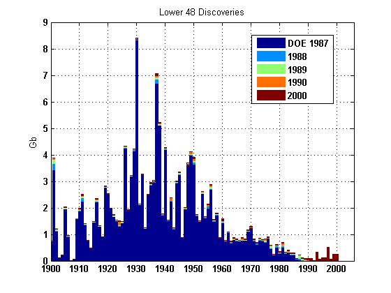
A peak at 2.5 would seem to ride at the lower edge of the noise envelope, whereas I see it riding higher, at maybe 3.5 average peak?
I am just guessing of course, and my prooblem is that I have not tried the N=6 power-law fit yet to USA, as I have been using just the Laherrere discovery data as stimulus which I reported on here:
http://mobjectivist.blogspot.com/2005/10/shock-model-applied-to-usa-lowe...
I also wonder if that number at 1900 messes with your least-squares fit, because I assume that number is a roll-up from the years before 1900.
http://pubs.usgs.gov/bul/b2172-f/B2172-F-508.pdf
It matches the data that Jean Laherrere send me. I used &lambda= 3 years in the Shock model so there is some spreading/smoothing of the resulting discovery curve.
I think that I found the potential source of the problem. I previously assumed that the initial volume was year 0 of reserve growth but it seems that it is year 1 of reserve growth. This offset has a big impact because most of the reserve growth occurs between year 0 and 1. The figure below is showing the impact of this offset on the estimated discovery curve + reserve growth.
But now it seems that I have too much oil with an URR around 322 Gb!
I guess this volatility is expected as the USGS reserve growth multiplier appears to approach infinity as you count back incrementally from one year towards zero. So this means that the USGS estimates are very sensitive to exactly where you start the reserve backdating.
Power law formulas, which the USGS use, exaggerate this effect even more as the slope of sqrt(t), or any t1/n where n>1, becomes infinite at zero as well.
322 Gb is a large error so that if we combine the initial year delta error with the infinite tail, I don't understand how the USGS can keep promoting this particular approach. I have had many problems with the censored data survival analysis that the USGS has used in trying to justify their extrapolations.
(1) They have to start using a model in their censored data analysis. They completely gloss over years that they have no data for and they think the censored data behaves exactly the same as the non-censored data.
(2) I think we have to calibrate to sanity checks, otherwise we will way overshoot the reserve growth estimates.
This is some data that I compiled a while ago from Attanasi of the USGS:

http://mobjectivist.blogspot.com/2006/01/grove-like-growth.html
At the time, I was trying to apply a diffusion-like growth and found that it fit a 1/x better (where x=time):
The interesting thing is that the 1/x behavior matches the Dispersive Discovery curve exactly at the beginning. This is easy to understand as cumulative growth is linear with time, yearly growth is constant, and therefore incremental growth goes as 1/Time! And the nice thing about Dispersive Discovery as well is that it has a finite asymptote.
But does this not limit the usefulness of discovery as a predictor for production since backdating of reserve size is generally based on production ?
http://www.guardian.co.uk/oil/story/0,,1405754,00.html
Just looking at the discovery curve and thinking about other discovery scenarios it does not look right.
Consider silver discovery in Nevada
http://en.wikipedia.org/wiki/Silver_rush
Given the greedy search concept we expect discoveries to increase rapidly as the searchers sweep a area then drop rapidly to a low level.
Your deb-ackdated discovery data has the correct form although probably not the correct numbers.
I would think that a discovery model would be robust and work for a wide range of reasonably hard to find resources.
It should work for mining, water wells, oil, rare plants, rare animals etc etc.
The point is the model can be developed against a lot of different data sets that may be cleaner than oil discovery.
To put the whole Climate Change issue into perspective vis-a-vis the Peak Oil Crisis, everyone needs to ask themselves, their associates, all sitting elected officials and those seeking office, especially the office of President of the United States, “What is more threatening in both the long and short terms, a beneficial 1 degree (F) rise in average world temperatures over the past 100 years, or a 1 percent decline in world oil production over the last 100 weeks - with steepening declines in the pipeline? Can our economy better deal with declining fuel inventories in an environment of persistent warming, or in an environment of declining average temperatures over the next several decades, the most likely scenario?”
This is odd, because I am tending toward the view that the climate system is running away from us and we could see 6C temperature rises by the end of the century.
And that would be far, far worse than the loss of all fossil fuels.
Have you read the reports by Carbon Equity?
http://www.carbonequity.info/
Nice Report, I'm going to have to go back through the calculus a few times before I fully understand everything. My one contention is the methane hydrates. If we were to start using methane hydrates we would be digging our own grave. Methane has 20 times more of an effect through radiative forcing on the climate than carbon dioxide. I believe some projections of the effect these methane hydrates in the ocean being dispersed into the atmosphere by warmer sea temps. can cause up to 5 degrees Celsius of warming. Economic losses from these negative externalities would make using methane in large quantities completely not as cost effective as one would think.
-Crews
I found your additional graph at this above comment most fascinating.
The red curve (find smallest fields first) is physically impossible because it would take an infinite number of years to exhaust the smallest fields first (i.e. those constituted by a few molecules of hydrocarbons trapped under some tiny pebble miles below surface).
The light blue curve (largest first) is physically difficult because what are the odds of not hitting a small field as you search for the next largest field?
Given those observations, of course the only realistic outcome is the one that walks the middle ground.
From a psychological viewpoint however, if the red curve had happened, people would have long ago stopped trying to find more wells because the EROI on the micro wells they keep finding up front is well below unity.
The blue curve must be psychological inverse in that people will keep trying to find more wells even as EROI drops below unity because their mental state will be, Gee we've always found big ones in the past --this must be a fluke and eventually we'll find another big one soon.
What's fascinating is that near the top right corner, the actual curve (dark blue) merges with the slope of the light blue curve. The actual response we hear from PO deniers is, "Gee we've always found big ones in the past --this current plateau must be a fluke and real soon we'll find another big one to save us and keep the party going." Moreover, they believe we're riding the red curve because "technology" will come through to help us find a new field that is bigger than anything ever discovered before. So they're flip flopping between the two unrealistic extremes instead of walking the middle path.
I think the red curve has a chance at being more realistic because it includes an acceleration in the discovery rate over time, which has to occur because of technology and a gold-rush mentality to seeking wealth.
WHT, You're saying that with tongue in cheek of course. Right? The internet does not covey tonality too well. ;-)
Seriously, the curve should exhibit an elongated S-shape. The data before 1920 will flatten and the data in recent years will flatten. That means the red curve to me looks more like an S than the turquoise curve. I guess the problem is that Khebab decided against putting in any inflection points on the two asymptotic limits and didn't include data before 1920. The turquoise will only look like an S if the inflection occurred well before 1920, which I don't buy. I don't buy that we haven't had an inflection point on the red either, but the shape isn't as counterintuitive.