| The Energy and Environment Round-Up: September 29th 2007 | The Oil Drum: Canada | The Finance Round-Up: October 2nd 2007 |
Modeling Oil Production to Estimate URR - Saudi Arabia, Kuwait and World
Posted by Stoneleigh on September 29, 2007 - 9:00am in The Oil Drum: Canada
This is a guest post by Apparent Peak. He started his career as an aeronautical engineer and is currently retired. Now he has more time to study peak oil and write posts for TOD. He has selected "Apparent Peak" for his handle which will become obvious once you have read the post.
1) Background
I have followed the subject of peak oil since the seminal article by Campbell and Laherrère appeared in the March 1998 edition of Scientific American. Approximately one year ago, I began to casually follow some of the discussion threads at TOD. The posts, the ensuing discussions and in particular, discussions on HL, logistic functions and Khebab's The Loglet Analysis caught my interest. I decided to investigate these topics since I did not know what HL was, let alone logistic functions. A quick trip to Wikipedia explained the Logistic function. As it turns out, it is a fancy exponential function that has characteristics similar to the Gaussian distribution.
Having read Khebab’s paper a few more times I realized that I did not have the patience to understand “successive Fischer-Pry decompositions”. However, one sentence in his paper was very insightful: “The Loglet decomposition is an elegant mathematical framework which consists in fitting a sum of logistic curves”. The idea of fitting a sum of logistic functions to model oil production made the process sound much simpler than successive Fischer-Pry decompositions.
More recently there has been much discussion regarding estimating a country’s URR using HL, Hubbert’s linearization, and especially the URR of the Kingdom of Saudi Arabia (KSA) and its potential oil production decline due to the depletion of the Ghawar oilfield (Ghawar reserves update and revisions by Euan Mearns and Depletion Levels in Ghawar by Stuart Staniford). To get a better understanding of the logistic function and its role in peak oil analysis, I decided to combine the concept of least squares with fitting the sum of multiple logistic functions to the oil production history of KSA as suggested by Khebab.
The least squares approach would provide a best fit to the country’s oil production and would address my curiosity to assess the quality of the results this method of analysis would produce. One of my objectives was to find another methodology that would complement HL and at the same time provide further insight into those situations that are difficult for HL.
2) Methodology
Calculating a least squares fit of a non-linear function is quite a simple and straightforward procedure using the “Solver” algorithm in Excel. Solver is designed to find an optimal value of a given “Target” cell that is related through formulas to other “Variable” cells. It does this by the adjusting/optimizing the variable cells until the desired optimum value is achieved in the target cell. For those interested in understanding how Solver finds the optimum solution, Excel provides the following note regarding its algorithm: “Microsoft Excel Solver uses the Generalized Reduced Gradient (GRG2) nonlinear optimization code developed by Leon Lasdon, University of Texas at Austin, and Allan Waren, Cleveland State University.”
For this exercise, by altering the parameters that define the individual logistic functions in the variable cells (Qo, the exponential constant and the peak year), the sum of squared errors in the target cell would be minimized. This methodology could be useful to interested TOD participants since Excel is well understood and readily available to many. The process used in this post is described below.
The logistic function for the cumulative production is given by:
Q(t) = Q0 / (1 + exp(-a(t – Tp))) (1)
Where:
Q(t) = Cumulative production to the year/time t
Q0 = URR or ultimate recoverable reserves
a = constant affecting the height to width ratio of the logistic function
t = calendar year/time
Tp = peak year, production peak for each individual logistic function
exp = the exponential function
The annual production rate P is the differential of (1) and is given by
P = dQ(t)/dt = aQ0 * exp(-a(t – Tp) / (1 + exp(-a(t – Tp)))^2 (2)
Units: Throughout this report, B refers to U.S. Billions, 1,000,000,000
3) Kingdom of Saudi Arabia URR: 160 B barrels or 260 B barrels?
The methodology described above was first applied to the Kingdom of Saudi Arabia’s daily oil production.
To model the KSA oil production, data was taken from the 2005 OPEC Annual Statistical Bulletin for the years 1938 to 2005. This data includes ½ of the oil produced in the neutral zone. The 2006 data point was taken from the April 2007 OPEC Oil Market Report. The annual KSA oil production data from 1938 to 2006 was input into Excel. Seven production rate logistic functions (Eq. 2) were then used to model the average daily production from 1938 to 2006. The spreadsheet (SA7_LS_Mult_Logistic), which details the KSA analysis and the results, is available to interested readers on request (from Stoneleigh(at)theoildrum(dot)com)
Since the Solver algorithm requires an initial guess to begin its iterative process, the logistic function parameters were adjusted to roughly approximate the KSA production history. It was this initial guesswork that indicated that six or seven logistic functions would be required to model the highly variable KSA oil production profile. Having set up the initial guess, the Solver algorithm was launched through the “Solver Parameters” window shown below to find the least squares solution.
The sum of squared errors, i.e. the error/difference squared between the actual and predicted production values, was placed in cell $M$8 in the spreadsheet and was specified to be there in the “target cell” box in the Solver Parameters window. Similarly, the twenty one parameters controlling the seven logistic functions were placed in the cell range $E$4:$K$6 in the spreadsheet and were specified to be there in the “changing cells” box. Solver varied the parameters in the cells $E$4:$K$6 until a least squares solution was found. By setting Q0 to zero and by changing the cell range in the “changing cells” box, the number of logistic functions desired/required in a given model could be varied.
Solver Parameters Window

Figure 1: Seven logistic model of KSA production
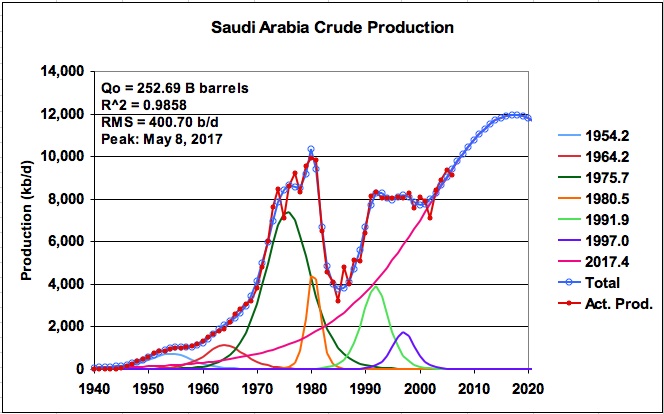
The first run using seven logistic functions yielded the following solution shown in Figure 1 (taken from Tab SA7-7-1 in SA7_LS_Mult_Logistic). It shows a URR of 252.69 B barrels and peak production of 11.94 M b/d on May 8, 2017. This solution is surprisingly close to the current Saudi Aramco claim on its website of proven oil reserves of 259.8 B barrels at the end of 2005 and its expansion plan of increasing production capacity to 12.5 Mb/d by 2009. Depending on the source, the question of whether the 259.8 is the URR or remaining proved reserves is still an ongoing issue.
The parameters that define each of the seven logistic functions in Figure 1 are given in Table 1. As can be seen, the logistic centred in the year 2017.4 dominates all of the other ones and accounts for 78% of the KSA URR.
Table 1: Parameters defining the seven logistic functions

Click to Enlarge
The predicted oil production profile follows the actual production reasonably well and the quality of fit can be assessed from the square of the correlation coefficient, R^2, and the root mean square error of 400.70 b/d.
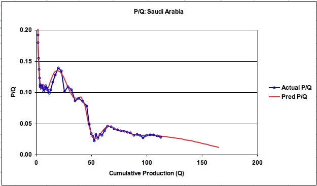
Figure 2: P/Q for KSA
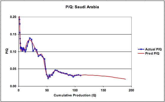
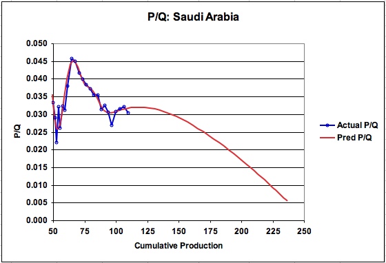
While this method directly provides URR, it is instructive to view the associated P/Q charts shown in Figures 2 and 3. As can be seen, the model predicted graph of P/Q follows the actual P/Q reasonably well and is not affected by the break in the linear portion of the curve at a Q of 96.7 B barrels. An expanded view of how the P/Q graph continues to curve down toward the URR of 252.7 B barrels is shown in Figure 3. Note that P/Q does not become linear until it passes Q of about 225 B barrels.
Figure 3: Expanded view of P/Q for KSA
Since this methodology uses an iterative non-linear least squares process to arrive at a minimum value for the sum of squared errors, the solution is a function of the initial conditions/guess. Consequently, the solution can only be described as a local minimum/optimum. Different initial conditions yield different solutions. It is necessary to vary the initial conditions to assess the sensitivity of the solution to the initial conditions and to determine the range of plausible solutions.
Having the first solution, the parameters in Table 1 were changed to find different solutions and to obtain a sense of the possible variation in the solutions. A number of runs were made. The results for two of the more extreme cases are shown in Figures 4 and 5 (Tabs SA-7-2 and SA-7-3). The runs produced URRs that ranged from 233.95 B barrels to 286.77 B barrels. Note that the quality of fit, as quantified by R^2 and the RMS error, is very similar to the run shown in Figure 1.
Figure 4: KSA daily production for a URR of 233.95 B barrels
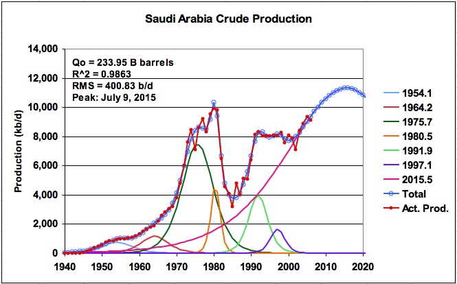
Figure 5: KSA daily production for a URR of 286.75 B barrels
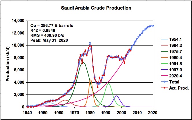
In reviewing the quality of fit of the model, it was noted that while the actual KSA oil production from the years 1998 to 2003 varied significantly, the model averaged the oil production variation over those later years. I wondered what would be the impact on the URR of trying to more accurately model the behaviour in the years after 2000. To do this, an earlier solution was modified by placing a small logistic function with a negative URR in the area of the production decline that occurred in 2002. The solver routine was then launched to find the least squares solution. The result was startling as shown in Figure 6.
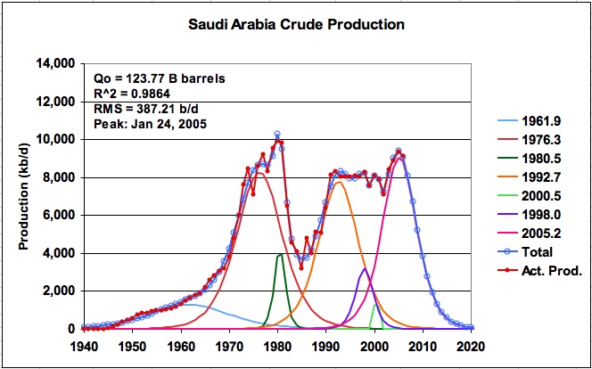
Figure 6: KSA daily production using negative logistic centred in 2001.9
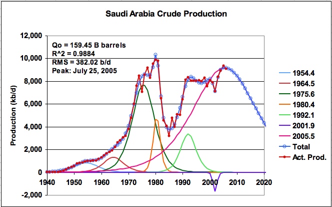
The URR decreases to 159.45 B barrels with a peak production of 9.176 M b/d on July 25, 2005. This is a reduction of approximately 100 B barrels from the earlier solutions. As can be seen, the model tracks the 2002 oil production excursion very well as quantified by the reduction in the RMS error to 382 b/d. Clearly the attempt to accurately model the years 2000 to 2006 has a profound effect on the URR and the future peak production date. This raises the question of how accurate does the fit need to be and where does it need to be accurate? The associated and expanded P/Q graph for this case is shown in Figure 7.
Additional cases were run using six logistic functions (SA6_LS_Mult_Logistic, also available on request) instead of seven and in general the URRs came into the 160 B barrel regime. Again the best fit was obtained when a logistic function with a small negative URR was added to one of the runs and is shown in Figure 8.
Some may question the merits of using a logistic function with a small negative URR in a model to predict oil production. However, the objective here was to treat the curve fitting of the production profile as a mathematical exercise to assess the impact of accurately fitting the profile over the years 1998 to 2004. The use of the very small negative logistic function was an expedient way to accomplish this. It should be noted that it is possible to create a decline in a profile by placing two positive logistic functions close together. This was done for clarity and the result is shown in Figure 9. This procedure results in a forced fit of the production profile in the last five years that gives an unrealistically low value for URR and a future production profile that appears to be unlikely at this time.
Figure 7: Expanded P/Q prediction with a small negative URR in 2001.9.
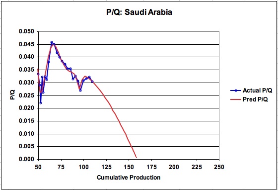
Figure 8: KSA production: 6 logistic functions (Note Tp = 0 for #1 logistic)
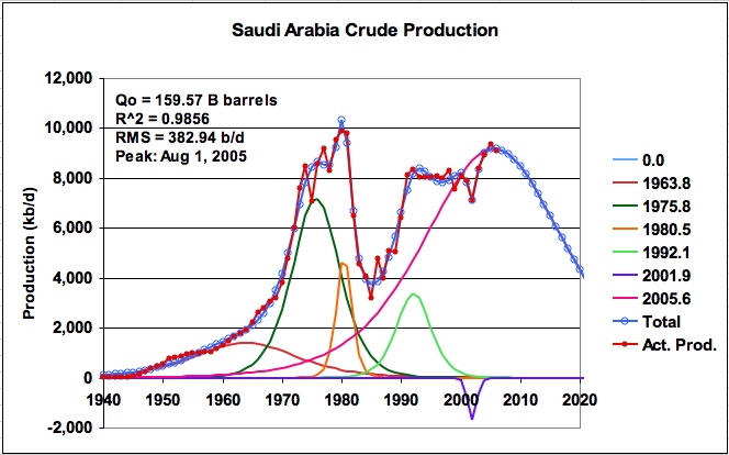
Figure 9: Effect of two Logistics to model the 2001 production decline
Another example of the difficulties and sensitivity associated with how to treat the last years can be obtained by projecting the average KSA oil production for 2007. The June 2007 OPEC Oil Market Report shows that for the first five month of 2007, KSA oil production has averaged 8553 Mb/d with a small increasing trend since March. If it is assumed that OPEC will not alter its target production until September and then permit production to increase in November and December, KSA could achieve an average production of approximately 8,625 Mb/d in 2007, if it increased its production by 250,000 b/d in the last two months.
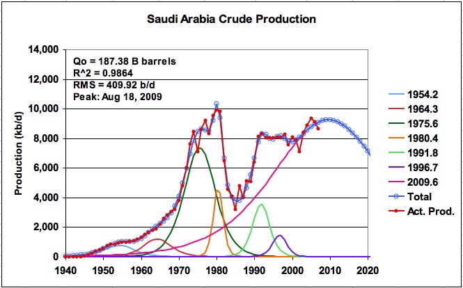
Adding this 2007 data point to the run that generated Figure 5, and using a model that averages the data over the latest years gives the result shown in Figure 10. Adding the projected 2007 data point reduces the URR by 100 B barrels to 187.4 B barrels and moves the peak production date forward to 2009. The P/Q graph is given in Figure 11.
Figure 10: KSA production with estimated 2007 production added
While it was hoped that this methodology could provide some additional insight into the URR of KSA, it only seems to have confirmed that there appears to be two possible solutions, either a URR of approximately 160 B barrels or 260 B barrels. Perhaps the KSA production profile is too difficult to model, whether one uses this methodology or Hubbert’s HL method.
Figure 11: P/Q for KSA production with estimated 2007 production added
On the other hand, we must recognize that the KSA production during the years 1998 to 2003 was constrained intentionally by Saudi Aramco to address market factors. Consequently, it might be reasonable to assume that the models that averaged the production during that time frame are more realistic than those trying to follow the profile exactly. The models that averaged the production data in those last years indicate that a URR for KSA in the range of 260 B barrels and a production peak of approximately 12,000 kb/d may be plausible. If KSA production were to exceed 10.5 M b/d to 11.0 M b/d in the next 2 years, it would lend more credence to the 260 B barrel estimate.
It will be difficult to assess the KSA URR until the reason for the production decline that began in March 2006 can be ascertained. It appears that the continuing excellent detective work by Staniford and Mearns regarding potential future KSA production will definitely be needed help to resolve the KSA URR mystery. We will need to know whether the decline is due to inevitable natural depletion or deliberately constrained production. If it is natural depletion, the URR estimate of 160 B barrels may be closer to the mark.
4) Kuwait
Another country of interest is Kuwait and in particular the issue of whether their oil reserves (URR) are 48 B barrels or 99 B barrels. In January 2006, Petroleum Intelligence Weekly (PIW) reported that Kuwait's actual oil reserves, which are officially stated at around 99 billion barrels, might be closer to 48 billion barrels.
Since there are two estimates for Kuwait’s reserves, modeling the oil production history would provide an indication of which estimate, high or low, was more consistent with the results of modeling. Also, since the production has been particularly erratic since 1970, including the decline to 185 kb/d in 1991 due to the disruption associated with the 1990 invasion of Kuwait and the ensuing war, it would provide another indication of the merits and limitations of this modeling methodology.
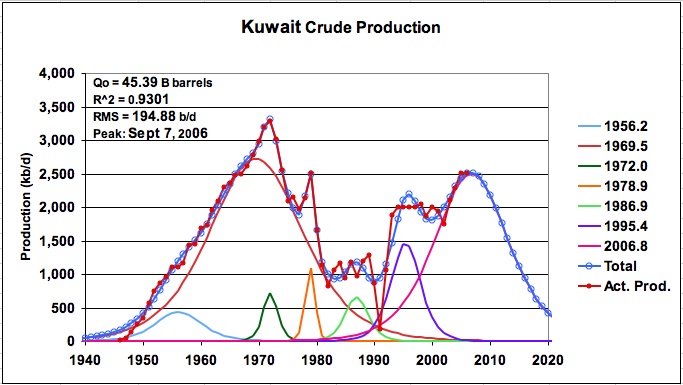
Kuwait’s oil production data was taken from the 2005 OPEC Annual Statistical Bulletin for the years 1938 to 2004. This data includes ½ of the oil produced in the neutral zone. The 2005 and 2006 production numbers were taken from the May 2007 OPEC Oil Market Report. Seven logistic functions were used to model the average daily production from 1938 to 2006 (SA6_LS_Mult_Logistic). The result is shown in Figure 12.
After running a few cases with similar URRs, the model shown in Figure 12 was selected because it attempted to average the production over the last 8 years. The model predicts a URR of 45.39 B barrels and peak production rate of 2.52 M b/d on Sept 7, 2006. This solution is surprisingly close to the PIW article that reported Kuwait’s reserves to be close to 48 B barrels. On May 15, 2007, the Kuwait Times published a similar article:
KUWAIT: More than half of Kuwait's oil reserves will not be produced through cheap traditional methods, Deputy Director General of the Kuwait Institution for Scientific Research (KISR) Dr. Nader Al-Awadhi said yesterday. Kuwait's oil reserves are estimated at about 95 billion barrels, among the biggest worldwide. Most production, if not all, is being produced through traditional methods, Al-Awadhi told a KISR workshop on "Managing Carbon Dioxide for Improving Oil Production" that started yesterday.
He expected that the traditional methods would produce 45 billion barrels, but could not be used for the rest (i.e. 50 billion barrels). Thus, emerges the necessity of developing new feasible environment-friendly methods for producing heavy oils, he said adding that oil production operations over the past years had focused on light oil.
Figure 12: Kuwait oil production
The Kuwait Times article appears to clear up the issue of the level of Kuwait’s oil reserves (URR). It states that the traditional methods would produce 45 B barrels and indicates that the remaining oil is classified as heavy. Since the oil produced to date has used conventional methods, the modeling can only infer its URR estimate from this historical production data. The article provides a degree of confirmation for the predicted URR of 45.4 B barrels for Kuwait and possibly its future production profile for conventional oil. Since Kuwait has stated that its Burgan oil field has peaked, it is possible that this means that its conventional oil production also peaked in 2006 as the model and data indicate. The interesting question that comes to mind from reading the Kuwait Times article is whether the Kuwait and KSA “anomalous reporting” of increased oil reserves in the 1980s is related to the discovery/addition of “heavy oil”. It is also interesting to note that Simmons in “Twilight in the Desert”, P174, in describing eastern Ghawar mentions a “massive tar mat up to 500 feet thick lay between Arab D oil and the formation receiving injected water”.
Figure 13: P/Q for Kuwait
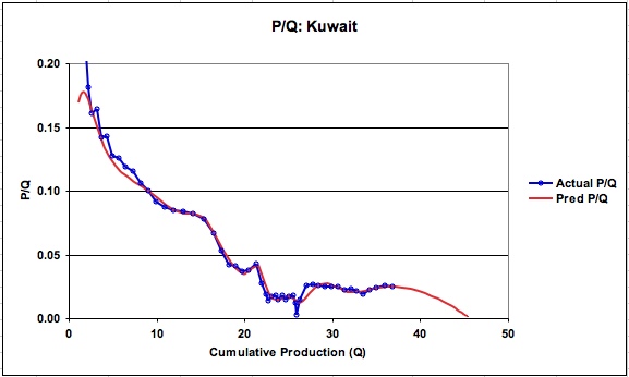
The P/Q graph for Kuwait is shown in Figure 13. As can be seen, there is a break in the linear portion of the data at a Q of 33.4 B barrels and one is left with the decision on how to deal with this using HL. The LS multi-logistic approach follows the break in the P/Q graph and heads for a URR of 45.4 B barrels. In this case we are fortunate to have the confirming statement from the Dr. Nader Al-Awadhi, “that the traditional methods would produce 45 billion barrels”.
5) World Oil Supply
On April 17, 2007, Khebab updated The Shock Model in The Shock Model (Part II). One of the points mentioned by Khebab in his post was the inability of the logistic function to address the 1970 to 1980 production bump. While this is clearly true for a single logistic function, the foregoing work on KSA oil production indicated that this would not be the case for a methodology based on fitting multiple logistic functions and decided to apply the same procedure as above to world oil production.
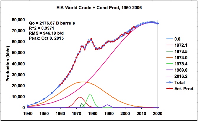
Figure 14: EIA World production for crude plus condensate (six logistics)
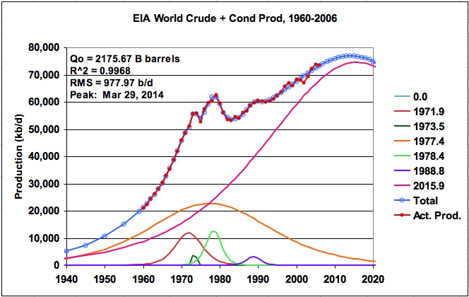
The data source for world oil production was the EIA International Petroleum Monthly sheet for crude plus condensate, t41d, supplemented with data from Table 1.2 from the Transportation Energy Data book of the U.S. DOE. Table 1.2 provided data from 1960 to 1969 and the May 8, 2007 EIA data sheet t41d provided information for the years1970 to 2006. Note that the 2006 data is the EIAs preliminary estimate.
Figure 15: P/Q for EIA world production for crude plus condensate
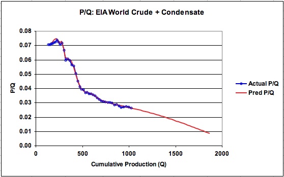
The EIA world oil production data was modeled using six logistic functions. As before, we are left with the decision of how accurately to model the 2000 to 2006 production profile. The initial runs were allowed to average the latest years. One of the runs is shown in Figure 14 and the results are given in Tab EIA World-6-1 (from EIA_LS_Mult_Logistic, also available on request). This model predicts a world URR for crude plus condensate of 2176 B barrels with a peak production of 76.9 M b/d on March 29, 2014. The associated P/Q graph is shown in Figure 15. Notice how the predicted P/Q graph has a very gentle downward curvature as it heads toward a cumulative production point of 2176 B barrels rather than the straight line which would occur from using a single logistic function.
Table 2: Parameters defining 6 logistic functions for world C+C production

Click to Enlarge
The parameters that define each of the six logistic functions shown in Figure 14 are given in Table 2. As can be seen, the logistic function centred in the year 2015.9 dominates all of the others and accounts for 80.4% of the URR.
To get an idea of the potential variation in Qo, additional runs using the six logistic function model with different initial conditions yielded URRs between 2120 B barrels and 2222 B barrels.
Figure 16: EIA world production for crude plus condensate (five logistics)
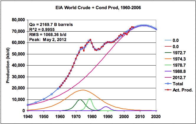
Applying a five logistics model to the production profile yielded the results shown in Figure 16. This model yielded a URR of 2169.7 B barrels. While R^2 was slightly lower, the RMS error was about 12½% higher.
Figure 17: World production for crude plus condensate (seven logistics)
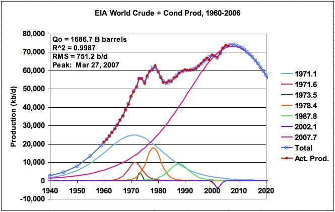
Again the lowest sum of squared errors was obtained with a logistic function with a small negative URR being placed at the year 2002.1. This seven logistic function model predicts a URR of 1686.7 B barrels with a peak production of 74 M b/d on Mar. 27, 2007 and is shown in Figure 17. Note that for this case, the URR is reduced by approximately 500 B barrels relative to the URR of 2175 B barrels shown in Figure 12.
As can be seen, multiple logistic models can follow world oil production very well and can address the 1970 to 1980 production bump along with the varying production profile during the years 1998 to 2004. However, one must question the validity of this result since a URR of 1686.7 B barrels seems too low, considering that Campbell, in the March 2007 ASPO letter, estimates the URR for regular conventional oil to be approximately 1900 B barrels.
The critical question that needs to be answered is whether the production profile in the years 2000 to 2004 should be averaged or modeled accurately. This is a rather critical question since the addition of the logistic function with a very small negative URR, which permitted a very accurate fit of the oil production profile during the years 2000 to 2004, resulted in a reduction in the URR of approximately 500 B barrels. As discussed in the KSA section, during this timeframe OPEC intentionally constrained oil production to address market factors. Consequently, at this time, the combination of the Campbell data and the OPEC production constraints suggests that a model that averages the data in the later years, rather than fits it precisely, appears to be more realistic and accurate for estimating URR and indicating future production.
The foregoing analysis has been focused on obtaining a realistic fit of the production profile using 5 to 7 logistic functions. However, in this type of curve fitting analysis, it is worthwhile to also investigate a looser or “averaging type” fit using only 2 logistic functions. This was not done for the KSA and Kuwait examples because of their non-logistic behaviour and the extreme variation in their production profiles.
The result of modeling the EIA data using two logistic functions is shown in Figure 18. This model increases the URR to 2244 B barrels and adds 69 B barrels to the six logistic model shown in Figure 14. However, it moves the peak date forward from 2014 to 2011. These two models are similar in that they both have one main logistic function to predict future production. The other logistic functions are smaller, track the deviations associated with historical crises and decay rapidly. By comparing the results from the “two logistic” model in Figure 18 with the very accurate fit using the “seven logistic” model shown in Figure 17, the six and five logistic models shown in Figures 14 and 16, respectively, can be considered as being a reasonable compromise between under fitting and over fitting the data.
Figure 18: EIA world production for crude plus condensate (two logistics)
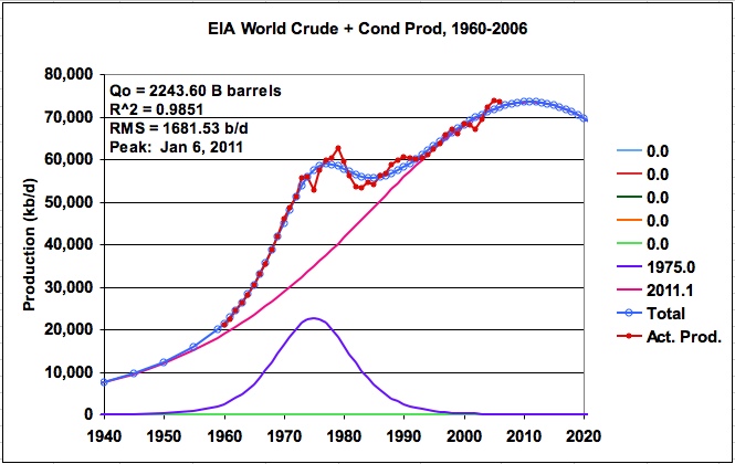
Figure 19: World production for C + C using the Gaussian distribution
While the above analysis was undertaken using the logistic function, it is worthwhile to note that it could have equally been done using the Gaussian distribution. A Gaussian solution is shown in Figure 19. While it is similar to that shown in Figure 14, the peak date is pushed further out since the shape of the largest Gauss function is not as “peaky” as the logistic function. It should be noted that the Gaussian distribution is not typically used for modeling resource depletion. However, Deffeyes, in his book "Hubbert's Peak The Impending World Oil Shortage", used the Gaussian to model U.S. oil production history and then continued to use it to model world oil production data.
6) British Petroleum Data for World Oil Production
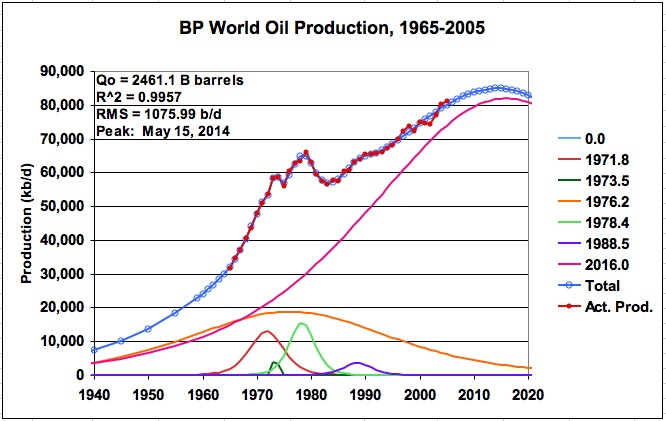
For a final example, BP’s world oil production data, which includes crude oil, oil sands and NGLs was modeled. The production data was taken from BP’s 2006 statistical review. Six logistic functions were used and the results are shown in Figure 20. The estimated URR is 2461 B barrels and the model indicates a peak production of 84.87 M b/d on May 15, 2014. While the peak production rate is different than that for the EIA C+C profile shown in Figure 14, due to the addition of the NGLs, the peak date is virtually the same when using six logistic functions.
Figure 20: British Petroleum’s data for world oil production (Six logistics)
Since the world oil production profile has a more regular nature, the BP data was also modeled using two logistic functions and is shown in Figure 21, Tab BP World-2-1 (BP_LS_Mult_Logistic, also available on request). This can be compared with the BP model in Figure 20, which shows a URR of 2461 B barrels. The 2 logistic model adds 138 B barrels to the URR, a 5.6% increase, and moves the peak date forward by about 20 months. As would be expected, the RMS error and R^2 are larger. The URRs of the two logistic functions are 119 B and 2480 B barrels respectively. Considering the simplicity of this two logistic model, it is not significantly different than the six logistic model.
In a recent paper by Phil Hart and Chris Skrebowski, they estimate the URR for world conventional oil and NGLs to be 2420 B barrels. Also the June 2007 ASPO letter estimates the URR for all liquids to be 2550 B barrels. The BP data modeled in Figure 20 shows a URR of 2461 B barrels, which falls in between these two estimates. While the all liquids data appears to be similar, it is not totally clear that the Hart-Skrewbowski data and the ASPO reserve data are reporting the same data as BP’s Statistical Review.
Figure 21: British Petroleum’s data for world oil production (Two logistics)
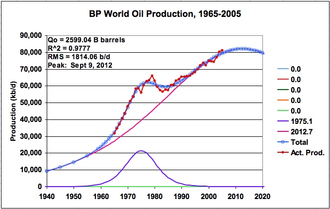
Figure 22: P/Q for BP’s petroleum data for world oil production (Two logistics)
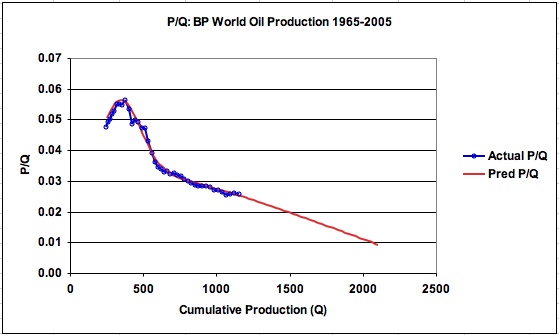
The P/Q graph for the two logistic BP model is given in Figure 22. As can be seen for this case, the projected P/Q is almost linear as would be expected for a case where there is one dominant logistic function that predicts future production.
7) Apparent Peak Oil
The foregoing analysis was focussed on estimating URR and when the peak in world oil production could occur using different modeling approaches (accurate vs averaging of latest years). The peaks ranged from the years 2007 to 2015. However, as the peak is approached and the annual change in the rate of oil supply decreases, another factor must be considered. In particular, it is necessary to consider the relationship between the annual supply rate of change (ROC) relative to the annual demand ROC.
Many are saying that world conventional oil production has peaked based on the EIA data for crude plus condensate shown in Figure 23. Recognizing that mandatory reductions in OPEC supply and additional difficulties in Nigeria are restricting production, it still may be too early to declare May 05 and Dec 05 as being the peaks for production of conventional oil.
Figure 23: EIA crude plus condensate monthly production
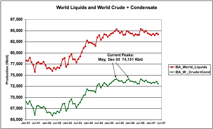
Nevertheless, the dramatic change in the slope of oil production from Jan 02 to May 05 compared to the production slope from May 05 to February 07, shown in Figure 23, does raise an interesting question/possibility. Is it possible that the world will see an “Apparent Peak” before the real peak is reached when supply cannot meet demand without an oil market correction? With supply and demand in relative balance as the peak is approached, the apparent peak could be defined by the point in time when the demand ROC for oil exceeds the supply ROC.
For 2007, the EIA is predicting an increase in demand of 1.6 % over 2006 while the IEA is predicting 1.8% increase. According to the IEA, the demand ROCs for the years 2003 to 2007 are 2.3%. 3.8%, 1.6%, 0.9% and 1.8% respectively. The average demand ROC for the last three years suggests that the supply graphs should be examined to determine when the supply ROC will begin to fall below approximately 1.4%. In the May 2007 edition of the U.S. Energy Information Administration “International Energy Outlook 2007”, it states “World use of petroleum and other liquids grows from 83 million barrels oil equivalent per day in 2004 to 97 million barrels per day in 2015. This represents an average annual demand ROC of 1.1%.
The annual supply ROC is plotted in Figure 24 for the three EIA cases that gave solutions for URRs between 2120 B and 2222 B barrels and peak years from 2013 to 2015. The ROC of the BP data was also calculated and it coincided with the URR 2175 graph.
Figure 24: Annual Change in the supply ROC for various URRs (six logistics)
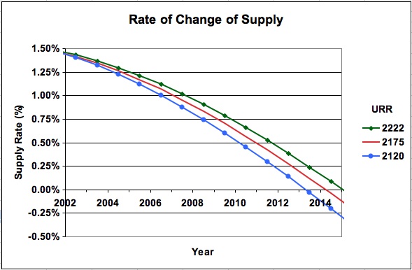
As can be seen, a supply ROC of 1.4% occurred around the year 2003 and during that time there was sufficient real world spare capacity to meet the even larger demand ROC of 2.3% that occurred that year. However, looking forward to the supply ROC for 2007 in Figure 24, it is between 1% and 1.1% for the three given URR scenarios. It drops below 1% after 2008. If the IEA’s and EIA’s 2007 tentative predictions for demand ROCs of 1.8% and 1.6% respectively are accurate, and the models developed in this paper are reasonable approximations for future real world oil production, the predicted gap between the decreasing supply ROC and the IEA’s and EIA’s projected demand ROC will either challenge the world’s ability to increase supply at a reasonable price or demand destruction will be required to balance supply and demand.
5) Conclusions
The above analysis has provided another curve fitting methodology to estimate the URR for a country or the world. However, the variation in results associated with the accuracy of modeling the latest years shows the necessity of having factual/better reservoir/geological knowledge to complement any modeling. From the above results for Saudi Arabia, Kuwait and world oil production, it is clear that good modeling requires a mix of good mathematics and physical data.
In the case of Saudi Arabia, along with many other countries, verified estimates concerning URR and reserve production capacity are not readily/currently available. Ironically, such information will likely only be made available after a country’s production has peaked; the fields have entered their irreversible period of decline; and reported oil production data from the IEA and EIA reveals the facts to the world.
While the issue of the dearth of information on oil reserves applies to many countries, the recent revelation from Kuwait regarding their reserves indicates this trend may change. As each country begins to meet the ever increasing challenge of trying to increase oil production against nature’s inevitable natural depletion, they will have to come forth with better production/reserve information.
While most of the modeling analysis focused on determining a country’s URR and the world peak production date, the analysis on supply ROC showed that the peak production date might not be the most critical time to pinpoint. A more critical time to pinpoint might be the “Apparent Peak”, i.e. the point in time when the demand rate of change for oil exceeds the supply rate of change. The results from the foregoing analysis show that there is the potential to reach the “Apparent Peak” in oil production beginning as early as this year, 2007, or possibly 2008. If we are now in this critical time period, the world’s ability to increase oil supplies at a reasonable price will be tested in a very short time or else demand destruction will be needed to balance supply and demand.
Personnel
Archives
- December 2008 (1)
- October 2008 (1)
- July 2008 (2)
- June 2008 (2)
- May 2008 (6)
- January 2008 (2)
- December 2007 (8)
- November 2007 (9)
- October 2007 (11)
- September 2007 (14)
- August 2007 (14)
- July 2007 (10)
- June 2007 (9)
- May 2007 (11)
- April 2007 (9)
- March 2007 (11)
- February 2007 (11)
- January 2007 (11)
- December 2006 (12)
- November 2006 (16)
- October 2006 (13)
License

This work is licensed under a Creative Commons Attribution-Share Alike 3.0 United States License.
Great analysis!
Your logistics analysis seems to reinforce the need for accurate URR estimates, as usual. Although, I think the lower numbers 'seem' to reflect the political realities we are witnessing.
IMO, your "APPARENT PEAK" concept has immense value and is reinforced by the realities of global interaction. The supply rate of change is slowing dramatically while the opposite is true for demand.
Even if we obtain a minor increase in production in All liquids in the next couple years...it will have to be offset by a dramatic decrease in demand BEFORE then...so the APPARENT PEAK(all liquids) is now or slightly in the past.
I have been looking at the IEA numbers for 2007. For the first 8 months the average production has been 85.1 M b/d. If production were to average 86.0 M b/d for the next 4 months, highly unlikely, the average for the year would be 85.4 M bpd. Production in 2006 was 85.16 M bpd. The projected 2007 production numbers would represent a modest 0.28% increase over 2006.
Perhaps, the more significant production numbers to be looking forward to are the December 2007 and first quarter 2008 numbers to get an idea of whether there will be any production growth in 2008.
I have a problem with using this approach.
It seems to me that one very quickly gets to the point of "over-fitting" the data. If there is an underlying reason why production might follow the sum of seven (or whatever) logistic curves, I wouldn't have the problem with the methodology-- say seven different producing reservoirs, each rising and falling according to your model.
As it is, the fluctuations in production follow various external events - global recessions, conscious raising and lowering of production at less than maximum production. I have a hard time seeing how fitting multiple curves to the data gives predictive value going forward.
I will agree that we will have a time when demand exceeds supply, perhaps prior to real peak. I think this has been called "Peak Lite" before; you are calling it "Apparent Peak". This is a real issue - we are probably pretty much there.
More than that, it seems that all that was achieved in this extraordinary work was the finding of the last logistic bell detected in each scenario (KSA KWT WORLD), but we don't know if those are the last curves we are able to produce.
That is, it doesn't tell anything about the future, because it pressuposes that these bell curves are all the last bell curves the world manages to produce, which I think it is rather unlikely.
And if you want to check what I said, I have more homework for you. Take all your KSA KUWAIT and WORLD charts, wipe out like 30 years and then try to plot the futures of it according to your method.
I bet that you will fail miserably in all of your predictions (probably except for the world, which is much more stable), which renders your theory moot.
Nice try though. That's the spirit.
Clearly this method cannot predict that a new Ghawar will be found somewhere. It can only infer a URR for all past and currently producing fields. I think that the URR results predicted for Kuwait and the World from the BP data speaks to the validity of this methodology. As for predicting the future, we shall have to wait to see how it evolves.
Ghawar was found in the first decades of the century. He places bell curves well beyond 1980, even after 2000, so I don't know what you're talking about.
I don't reckon "ghawars" to have been found since, but north fields, and now tar sands, shale oil, perhaps helped making those bumps.
But there is a race towards artic oil, if I remember. And Angola is making huge increases.
Either way, doesn't matter. This is numerology, not science. It tries to see simple patterns on a very complex structure. How could it possibly go wrong? Correlation... you know what.
Even King Hubbert didn't calculate URR with his own HL curves. He was not that dumb.
Pff. Almost everyone agrees that we are close within the peak. So that's not rocket science. What science is this that creates a span between URR of KSA of between 160bb and 260bb?!? Is this thing even useful?
I also don't think so.
It's a good try though, and I commend the spirit. Not the results, not the science.
The comment regarding Ghawar has nothing to do with placing bell curves beyond 1980 or 2000. The least squares process determines the size and position of the logistic functions that are required to model KSA's multi-peak production profile.
The Ghawar comment was intended to indicate that I, along with many others, do not believe that a new oil field the size of Ghawar and capable of producing 6.0 M bpd or multiple queen fields will be found in the future.
As for Canadian Oil Sands, they are already accounted for and their rate of production increase will be slow. As for shale, that production may show up after the peak year.
On one hand you are looking at oil sands, arctic oil, and Angola making huge increases to perhaps helping to make additional production bumps. On the other hand, you say almost everyone says we are near the peak. What is your position?
You ask the question “What science is this that creates a span between URR of KSA of between 160bb and 260bb?!?”
First off lets consider the real world situation. Saudi Aramco claims 259.8 B barrels proven oil reserves at the end of 2005 on its website and describes its expansion plan of increasing production capacity to 12.5 Mb/d by 2009. Many TOD participants and others believe that that the KSA reserves are closer to 160 B barrels. Isn’t it amazing that this “numerology” gives two answers, one in the 160 B barrel range and the other in the 260 B barrel range, that reflect the current debate occurring in the real world.
This numerology also indicates what to look for in future KSA production to get an indication of the real URR. For the 260 B barrel estimate to have credence, the numerology shows that KSA production would have to exceed 10.5 M b/d to 11.0 M b/d in the next 2 years. With the IEA indicating that world demand is increasing at around 2% per year, KSA’s ability to increase production to its claimed levels may be tested soon.
You have looked at the KSA results and question the value of the two results. At the same time, you have chosen to ignore the accuracy of the Kuwait and BP results. The projection of a URR of 45B barrels for Kuwait is spot on with Dr. Nader Al-Awadhi statement that traditional methods would produce 45 billion barrels. The BP results, which show a range of 2460 B barrels to 2600 B barrels for world URR, are also in close agreement with the latest projections from Hart and Skrebowski on world URR of 2420 B barrels and the varying projections in the range 2500 B to 2600 B barrels in ASPO newsletters #73 to #80.
As I mentioned in my reply to Gail the Actuary, I am following in the footsteps of many TOD participants who have gone before me looking at past oil production to get some insight into future production. Since others have also been making models and projections on TOD, I am trying to understand the nature of your concerns.
Are you addressing the use of analysis in general? Are you addressing the value of analysis that uses a number of logistic functions to model multi-peak production profiles, such as the use of loglets in the Fischer-Pry decomposition, which is a challenge for many curve fitting techniques? Are you addressing the use and ability of the “least squares method” to fit a number of logistic functions to model multi-peak production profiles?
And my comment was intended to indicate that the lack of appearance of new "ghawars" was definitely not a reason for the lack of future production bumps, as if that was the case being, then there would be no bumps in the 1990's and 2000's.
I look at the world, not at my crazy numbers and a way to correlate them nicely into a chart. I look at the world and see further bumps that would add to your final big bump in the future, so that the final curve would be the sum of those future bumps and that last bump of yours. It could even be another negative bumps, like those you've used.
I see then that these predictions are worth zero, they only indicate a good correlation in past summed curves. The only way this theory could be of any use would be if one could know if further bumps are possible and produced, and how much. THEN, one would HAVE to add those curves to the last one in blue in all of those charts.
You would by then have your own PREDICTION.
OTOH, I say we are almost or past the peak. That is obvious and doesn't come from this analysis, rather from many others that didn't depend on curve fitting (HL comes to mind), numerology or astrology.
Amazing indeed. But it is rather like watching the horoscope that says that it is about to rain, but then again it may not rain. How that kind of knowledge is worth anything is beyond me. I couldn't care if it was astrology or numerology, if it told me exactly what was going to happen RATHER than telling me exactly what I want to hear, then I would gladly accept it. But it doesn't.
STILL, it is only numerology. Period. Even stopped clocks give always too good answers (160 and 260?) everyday.
...Which renders your theory, among many others moot. You are not considering many things, like politics, specific geological problems, human error, worldwide actions/reactions, wars, etc. You just plot the line and tell us "if x doesn't reach y in z time, then abracadabra". That's nonsensical analysis. Even if your numerology is somehow based on a much more fundamental phenomenon, you can only aspire to a certain curve fit that doesn't wipe out the noise. And this noise could falsely trace you to the final URR between 160 and 260. This means that even from two years now you can't tell final URR of KSA. You can only guess, or aspire to know.
You could eventually be very wrong.
Which is to say that a newly created theory has achieved to bring on the same results that we've already known / suspected. Brilliant. That is not enough. Learn more of Scientific Method: that is not enough.
I know nothing about Fischer-Pry. I am addressing to your charts and to this simple reasoning: you took all of your charts and fitted bell-shaped curves with "least squares method". Fine. You then, show us your bell curves, they are a lot. Then, you plot a final one, blue painted, which is always given as the final curve, the final bell shaped curve, and yet you don't give any reason for us to take that blue curve as the final curve of history in oil production, you took that from granted. That's what I question and what seems to me as the greatest flaw.
Because, you see, a great way to see if your theory has any predictive value, is if you do what I challenged you to do: wipe out years to your plots (in several different charts), trace back your curves, and let us see if your charts always tells the same story. I bet they don't, I bet they always tell a different URR, a different story and different bell curves.
I am not against "analysis in general", as I commended the spirit of it. I like what Hubbert made. But he made a different approach. He didn't use curve fitting to predict URR. He made the other way around. That's why I called this "numerology".
I think that we are going to have to agree to disagree on the merits of this post.
I am following in the footsteps of many TOD participants who have gone before me looking at past oil production to get some insight into future production. I would agree with you that external events affect the production profile. However, countries have been producing oil for many years and I guess some of us believe that external events should not dissuade us from the challenge of analyzing past production to predict the future. Check Khebab’s latest post on September 22, 2007 to see the range of analysis and predictions. Also, while the external events have a large effect on a single country, they have a much smaller effect on world production.
Previous posts on TOD have attempted to model past production using different approaches, i.e. loglets, successive Fischer-Pry decompositions, etc. All of these approaches result in a number of logistic functions fitting past production to gain some insight into plausible future outcomes. Being familiar with least squares, I decided to try a different approach, i.e. directly fitting a number of logistic functions to the production history using the well known least squares approach and Excel. I also was interested in seeing whether the results would provide greater insight into the HL method and when it can be used.
As you have noted, one can over fit the data. On the other hand, one can also under fit the data. It is a decision that to some extent is determined by the variation in the data being fitted. The KSA and Kuwait data were quite variable, very non-logistic, and I used 6 and 7 logistic functions to model these cases. The more critical issue, as discussed in the post, is how accurately to treat the later years. Some of the results speak for themselves. The projection of a URR of 45B barrels for Kuwait compares well with Dr. Nader Al-Awadhi statement that traditional methods would produce 45 billion barrels.
Looking at the results, you will note that the early logistic functions are small and decay quickly. Their main purpose is to unload the last logistic function so that it can do a better fit on the later years.
For the EIA and BP world production data, I addressed the question of over fitting and under fitting by showing results using 6 and 2 logistic functions. For the BP case, the difference between the two results was 5.6% on the URR and a shift of 20 months in the peak. This gives an indication of the low sensitivity of the results to the number of logistic functions used when the production profile is close to being logistic. The two and six logistic BP result are interesting because they are in close agreement with the latest projections from Hart and Skrebowski on world URR of 2420 B barrels and the 2600 B barrels projection in the ASPO newsletter #80.
My ultimate aim was to study the relationship between the annual supply rate of change (ROC) relative to the annual demand ROC near the peak to see whether we might see an apparent peak, or as you mentioned “Peak Lite” (New to me). For 2007, the results indicate that we should be seeing a supply ROC of less than one percent. Looking at the latest IEA data, I will be surprised if the 2007 production is more than 0.5% larger than 2006.
I do quite a lot of non-linear least squares fitting and I try to stick with Bevington's CURVEFIT as often as possible because the systematics are understood by quite a few people. I'd be interested to know the genetic relation between this program and the one you use.
I have to agree with Luis, that if you know that the main current production comes from a field that was recently discovered, you would do best to include this in some way. Before I read his post, I had been thinking that you might want to add a technologically learning curve enabled huristic by insisting that the widths of you curves decrease with time. People know how to suck a field dry faster as they gain experience. With non-linear fitting you can do all sorts of things like this and you don't need to actually work out the partial derivatives any more because of how fast computers run now. (I expect that this is what your program does.) On the other hand, adding in interesting constraints can introduce degeneracies that inhibit convergence or make it impossible using a stright forward gradient approach. To deal with this I will go to the AMOEBA program given in Numerical Recipes which will not sucumb to this problem. I expect that you could make the width of your functions a simple function of their time centers or simply rescale the time axis and use fixed width functions in the rescaled axis and you would not see large issues with degeneracies.
It is worth remembering that daily production is likely to be very correlated so that your number of degrees of freedom may be much lower than the number of data points would indicate.
If you need help including constraints in your fitting, I'd be happy to try to assist.
Chris
I think for the first time I'm actually clearer maybe :)
I think a simple linear weighting is enough at least for a first pass. I like how your saying decrease the widths of later curves but don't you get the same result by using a global linear weighting that weights early data above late.
The slope of this line is effectively increased product rate vs enhanced URR. I'm suggesting that 2:1 is a reasonable guess.
Its effectively the same and simpler.
From the article:
a = constant affecting the height to width ratio of the logistic function
If you make a=a(Tp) then you can constrain the width to be a function of time. It seems to me now that reparameterizing t will leave you leave you with a curve that is not the logistic curve in actual time. So, to keep it a sum of logistic curve you'd have the width vary by a factor of two or three perhaps.
As you can see from the equation for P (there is a closing parentheses missing in the numerator), ingnoring the constants, it peaks at a value of 0.25. The half width therefore occurs at a value of 0.125. Application of the quadratic equation give -a(t-Tp)=ln(3+2sqrt(2)) or ln(3-2sqrt(2)) so a=2*ln(3+2sqrt(2))/delta_t year^-1 where delta_t is the desired half width. If we assume that drilling equipment in a country is obtained at a constant rate and is repairable so that the capacity to drill increases with time then we might be motivated a little to rise to peak at least on a shorter timescale as more equipment is accumulated.
I don't think weighting would act as much of a constraint on the halfwidths of the components.
Chris
Okay got you.
I agree with you thats a nice analytical way to do it.
Non-linear least square regression programs I'm familiar with let you apply weighting functions a number of ways.
The weighting function would be this ?
So the weight is increased drilling equipment and better technology which can be treated as the ability to drill more wells since this model is not taking into account the physical limitations of how closely spaced well are this is in the data.
So its a linear increase in well drilling capability to start with we could simply use rig counts. Later this saturates and then technical advances make a rig more powerful but for a first pass a simple analysis using rig counts makes sense.
So a normalized weighting by rig count seems pretty reasonable.
Note this goes right to my assertion in the past the the logistic fit is arising from the birth and death of wells.
If this is true a dependency on the "birth mothers creators" or oil rigs makes sense.
This correct will correctly discount later drilling efforts around the peak and post peak since more of the URR will be correctly weighted back on the earlier well data.
The only flaw is you have a undercount past peak where rig count stays constance or declines but technological boosts continue. The earliest data when their are few rigs may also be noisy.
Is the number of active rigs available for the US and is split between gas and oil ? My understanding is a lot of the data does not differentiate between gas and oil drilling.
If not I bet we have good numbers for the North Sea ?
Data anyone ??
I think we have demonstrated that the use of Logistic-styled curves precludes us from ever trying to model the generated profile in terms of real-world analogies like rig count. As Khebab put it succinctly in other posts, we can either (1) curve fit or (2) use a model.
This post by Apparent Peak is impressive but it remains curve-fitting.
I will bring this up again, but the minute you invoke a birth-death model on oil production via rig count you will run into the contradiction of Current Carrying Capacity != URR. Deaths in the birth-death model remove entities from the Current Carrying Capacity but they cannot remove anything from the URR because URR is cumulative (while carrying capacity is not).
See this post, "Logistic Model for HL purely a Birth Model"
http://mobjectivist.blogspot.com/2007/09/logistic-model-for-hl-purely-bi...
Its all a matter of matching variables if the focus is on wells and well production when a well is capped the carrying capacity is reduced. I.e the field cannot have more wells.
So I would say capping a well can easily be mapped to a death and whats lost is the capacity of the field as far as how many wells can be drilled.
If its really about wells which it seems to be its more about how you can extract the oil. In time the number of places you can drill a new well drops and thus the carrying capacity drops.
The terms used in the Logistic equation URR/Production rates are simply proxies for the underlying physical real logistic process of well creation death and loss of places to drill or carrying capacity.
I'm not sure why your mapping the logistic equation back to oil itself I've not proposed this. I don't think it has anything to do with oil it has a lot to do with exploitation of a resource in the case of oil this is wells and prospects for drilling more wells.
I'm mainly interested in a fitting method and applying constraints. When I saw the shape of the data, it seemed to me that a narrow function with large amplitude might do something that looks a little like the recent data, and after reading Luis comment that a big field was tapped recently and seeing the video saying that the same field is in decline I thought a constraint that makes production from new fields faster than production from historic fields might have a physical motivation. I don't have a big stake in the idea that this might be predictive. I'm willing to accept Richard Gott's method of prediction. We've been using oil for about 80 years so there is about a 75% chance that we won't be using it in 240 years. And, I think that there is real predictive power in looking at the pattern of discoveries of oil fields. My comments, though, are more about trying a few things in fitting.
Chris
Let me parse one of the statements you make:
You say the "terms used in the Logistic equation ... are simply proxies for the underlying physical real Logistic process". This reads like a tautology. Did you really mean to say this? Because when I read it, it looks like you are saying that the real physical process follows the Logistic equation.
But then you say this, in responding to me:
This statement completely contradicts your tautological statement preceding it. You, not I, are proposing this.
Good catch and a sharp eye for noticing that missing bracket Mdsolar.
Thanx
No sweat. When you said it was the derivative that was info enough. It is kind of a pretty function. Symmetric without the heavy handedness of the Guassian. I use the error function to fence parameters sometimes to get well behaved convergence but implementations are dicey because it is an indefinite integral. I might switch to the logistic curve for this purpose.
Chris
This is my first crack at non-linear curve fitting and I am not familiar with Bevington's CURVEFIT and do not have access to any high powered NL programs. I just set the program up in Excel using equation 2. Having the predicted values and the actual values I calculated the SS and then launched the “Solver” algorithm in Excel and let it find the minimum.
I had to use different initial guesses to obtain an idea of the stability of the solution and in general there appeared to be a lot of local minima over a relatively flat range. When I added an initial guess with a small negative logistic, which converged to -1.2 B barrels, as shown in Fig 6, there was a staggering drop of approximately 100 B barrels in the URR and a major reduction in the SS. This then raised the question of how accurately to fit the later years?
From the short description given in Excel, the Solver algorithm appears to be a type of relaxed gradient approach. While I understand gradient methods, I am not familiar with their intricacies and pitfalls. I was just thankful that such a powerful tool was available in Excel. How does Bevington handle multiple valleys? Does it search for the lowest one?
I will review the comments from the other TOD participants regarding the addition of a technology component. As you can see, there are already concerns being expressed regarding over fitting.
With regard to the comment “I have to agree with Luis, that if you know that the main current production comes from a field that was recently discovered, you would do best to include this in some way.” I am not aware of any data set that is available from a recently discovered field that could be subtracted from the world production and treated as a separate sub-data set.
I would be interested in having further discussions regarding this methodology and how Bevington could add to it. Send an email to Stoneleigh, the publisher of this post and who has my gmail address and then we could communicate off line.
Like Gail I am worried about over fitting.
A test of whether this close fitting has any predictive superiority over a single logistic is to truncate the time sequence at some point in the past, produce a fit of the remaining data and see if it produces a better prediction of the truncated data.
My shared caution about over-fitting is in part due to the fact that Fourier analysis will give a fit to any continuous finite single valued function. This includes a set of time functions that are identical up to a certain point (which could be the present time) and thereafter diverge strongly.
There are many functions beside sinewaves that can be used for such fitting. Logistic curves may not have the required orthonormality to fit any curve but they can fit a great many.
In reply to a previous comment about over-fitting Stuart Staniford described it is as "pure epicycles" recalling the efforts of early astronomers trying to fit the motions of the planets to a earth centred universe by fitting epicycles onto epicycles onto epicycles.
Making a assumption of the logistic curve for fitting in the first place is claimed to be over fitting by many :)
I think this approach has merit and the number of knobs to turn can be reduced once we have a good reason to reduce them.
Right now it has a constraints problem that needs to be solved. We have no way to constrain the number of curves. So its not clear how to back down from the "over fit" condition.
In other posts we are suggesting one constraint based on active rig count.
So first lets see if a few reasonable constrains can help reduce the "over fit".
As I have set up this methodology, I can select from 1 to 7 logistics to model the production history. For the strongly variable non-logistic cases of KSA and Kuwait, I have tried 6 and 7 logistics. For the closer to logistic cases of world production, I have shown solutions for 2, 5 and 6 logistic fcns.
As I have noted in the post, my big issue is how to treat the latest years, average them or fit accurately. At this time, I believe that averaging is more realistic since in a few cases the accurate fit gave an unrealistically low URR. See Figure 17.
I tried one logistic fcn and it was very bad because I did not have sufficient data before 1960 to anchor the left hand side of the logistic fcn. Clues on where I can get earlier data on world production would be appreciated since I would like to see what one logistic can do. Also I am looking for data on Russia.
The early logistic fcn are small relative to the last one and decay quickly. As far as I can figure out at this time, their main purpose seems to be to unload the last logistic function so that it can do a better fit on the later years.
Yeah it has some problems but also quite a bit of merit.
Although it is curve fitting the key to curve fitting is generally to use real variables to control the constraints and as data filters.
My suggestion is to center your logistics on wells drilled per year. This is fairly close to some of your better fits.
As the price of oil drops drilling activity drops and future production "declines".
I really think your on to something with your approach and it seems to be suggesting and additional factor is at play.
1.) The obvious reduction in immediate output during embargos or price collapses.
2.) The secondary effects on drilling and investment activity and thus future production. So a short term event echo's for quite some time through the production profile.
3.) This leads to a rise and fall in production capacity and rate of expansion which determines future production rates.
4.) The depletion effects fields no longer worth drilling this increases linearly with time so the number of wells drilled decreases naturally as you simply run out of places to drill.
In any case if you agree its all about well which makes sense since the cost of a well is constant regardless of its production rate. Dry holes do not come with a discount. The actual oil/gas production rates are just proxy data for well drilling activity and success rates.
Its really not the oil and gas industry its the oil well and gas well industry. The don't call the mining industry the metal industry. We have no problems focusing on the expense of extraction for other materials like coal and metals but for some reason for oil the mining costs are swept under the table and the focus is on the production rate.
In any case thats for your work its given me more to think about which is why I can't resist the oil drum.
"My suggestion is to center your logistics on wells drilled per year. This is fairly close to some of your better fits."
Wells drilled is not an independent variable. Tautology alert?
As I mentioned in my response to Gail, one can over fit the data as well as under fit. It is a decision that to some extent is determined by the variation in the data being fitted. The goal is to find the right balance. In the case shown in Figure 17, it was obvious that over fitting was the case since it gave an unrealistically low URR.
The more critical issue, as discussed in the post, is how to treat the later years. Based on the results in Figure 17, I think that averaging is the more appropriate approach.
However, some of the results speak for themselves. The projection of a URR of 45 B barrels for Kuwait compares well with Dr. Nader Al-Awadhi statement that traditional methods would produce 45 billion barrels. Also the BP results for 2 and six logistic fcns, which show a range of 2460 B barrels to 2600 B barrels for world URR, are also in close agreement with the latest projections from Hart and Skrebowski on world URR of 2420 B barrels and the varying projections in the range 2500 B to 2600 B barrels in ASPO newsletters #73 to #80.
I question the loglet analysis' predictive properties. It seems like a simple curve fit with the most weight being given to the highest, flattest, most recent points.
There is always that fundamental question of whether the past can predict the future. As I have noted above, predicting future production from past production is a favourite pass time for some TOD participants.
The least squares method of fitting logistic functions gives equal weight to all of the data points. The more critical question that needs to be answered is whether the world production profile in the years 2000 to 2004 should be averaged or modeled accurately. Based on the results from doing it both ways, I felt that averaging was the better way.
The URR results predicted for the World from the BP data and for Kuwait from its data speak to the validity of this methodology. The BP results for 2 logistics predict a world URR of 2599 B barrels. The ASPO newsletter #80 predicts a URR for all liquids of 2600 B barrels. Can this be just coincidence?
Freeman Dysan
Doing an analysis is always worthwhile since it does provide insight, regardless of the number of parameters used.
AP,
Of course, no offense intended, but its a great quote ;) I vaguely remember wavelet theory from Uni, but then we were fitting "hat functions". I recall we had to show "condition O" - that the basis functions were orthogonal in the sense that sin and cos are. Do logistic fcns satisfy this? Wavelet analysis says that the hats have to be "harmonics" in both frequency and amplitude. Have you tried to do this?
There was a tie-in with Shannon theory. That if you could produce an efficient wavelet compression, then in some sense you could say that you had the most "succinct" representation of the data, and that the co-efficients meant something real about the underlying process.
And thats all I can remember about that.
I did not encounter wavelets in my days at U or practicing aerodynamics and so I never thought of trying to use them. I guess that one could consider the oil production profile to be an irregular hat and wavelets might to the trick. It sounds like loglets followed wavelets.
We just used S and C functions to calculate F series expansion coefficients at U. That O condition was clever since it made the calculations much simpler when we only had slide rulers. With Excel, I don't worry about O.
The logistic function is not orthogonal since it is only one sided. As I vaguely recall, to get that O condition, the function had to be oscillatory. As for Shannon, I always thought that’s a nice place in Ireland.
Take care and have a great day
Nice finally someone does some non-linear least square fits.
One thing that your analysis might be bringing out is the technology effect. Not that I think you meant to do this but it seems capable of exposing the role of technical advances.
Basically it seems to me that technology has allowed us to double the rate of production for a given type of field over about the last 30 years. Given your analysis and if you had data say in the GOM of similar fields developed over a broad time span with production rates and URR's we probably could get a empirical measurement of the "technology effect".
If you add this to your analysis as a constraint then I think you will find the higher URR estimates can dismissed. The idea is I think this method could actually correct for the technology effect. And its exactly these technology effects that are used to claim higher URR. You waited production equally and I'm saying that you need to place higher weights on earlier production than later with a simple linear weighting scheme before doing the sums.
The pust the value of the earliest oil produced at about twice todays. Another way to say it is its the easy oil effect.
This is one reason I'm convinced we will see decline rates post peak that many will find surprising.
Hi Apparent Peak, this is an interesting post, and educative too.
A few folks have already pointed out the weaknesses of this kind of analysis - and especially in the case of Saudi - the way it looks so deeply to fit closely the past, turns up not explain much about the future. Anyway Saudi is a very special case.
I'd rather focus into the interesting things we can learn from this post. When considering the world situation, even sending the heavy cavalry against it, we get a single cycle dominating the current setting. Using 7, 5 or 2 cycles the picture doesn't change that much.
That was more or less the result we got from Khebab's Loglets. A key point to understand about this, is that for the last 20 years or so the world oil consumption per capita has been flat.
Hi Luis!
Yes, KSA is a very special case and we are going to have to wait a few more years to get an answer. As I mentioned in the post, it appears that the continuing excellent detective work by Staniford and Mearns regarding potential future KSA production will definitely be needed help to resolve the KSA URR mystery. However in the mean time, I have come to realize that the KSA results are giving the same results as we are seeing in the real world.
On their website, Saudi Aramco claims 259.8 B barrels proven oil reserves at the end of 2005 and describes its expansion plan of increasing production capacity to 12.5 Mb/d by 2009. Many TOD participants and others believe that that the KSA reserves are closer to 160 B barrels. Isn’t it amazing that this least squares method gives two answers, one in the 160 B barrel range and the other in the 260 B barrel range, that reflect the current debate occurring in the real world.
The results also indicate what to look for in future KSA production to get an indication of the real URR. For the 260 B barrel estimate to have credence, the projection shows that KSA production would have to exceed 10.5 M b/d to 11.0 M b/d in the next 2 years. With the latest IEA estimates indicating that world demand is increasing at around 2% per year, KSA’s ability to increase production to its claimed levels may be tested soon.
Very good work. Our previous contribution to the debate:
http://www.energybulletin.net/16459.html
Texas and US Lower 48 oil production as a model for Saudi Arabia and the world
Jeffrey J. Brown & "Khebab", GraphOilogy
Note that in the our article, I never claimed that the pre-peak Texas HL plot, which is quite noisy, could accurately predict the peak. I did claim that the total HL plot gave us an idea of at what stage of depletion that Texas peaked. And, given the more stable Saudi HL plot, we should then be able to predict a time frame for the Saudi peak, resulting in the conclusion in our article (based on production data through the end of 2005).
I have gone back and looked carefully at the pre-peak Texas HL plot (Texas peaked in 1972), and I think that there is actually some useful information there. (I think that the probable Texas URR is in the 66 Gb range.)
If we just focus on the 1957 to 1965 data, there is a strong linear pattern, pointing to a URR estimate of about 50 Gb. If we include the 1965 to 1972 data (the infamous "dogleg up" pattern, which appears to be an artifact of a swing producer going to 100% of productive capacity) we get a wildly improbable URR estimate of about 110 Gb.
Therefore, the prior swing producer data suggest that we should discount the recent "dogleg up" in the Saudi production plot.
If we then consider the fact that Saudi Arabia now, like Texas after 1972, is showing the following characteristics: rising oil prices + increased drilling = lower oil production, I think that the most likely scenario is that the lower estimate of Saudi URR is the most accurate.
BTW, the key test of whether or not Saudi Arabia has peaked is not if they can show a few months or even a year or two of rising production, we have seen that in Texas and the overall US. The question is, will they ever exceed 9.6 mbpd in crude oil production in a given calendar year? IMO, the answer is no.
From our May, 2006 paper:
The infamous dogleg is and obvious example of technology distorting URR in the case of texas it was simple drilling of a lot more wells. A more subtle effect is increased production over time giving a inflated URR for production later in time as production methods increase.
Balancing this of course in enhanced recovery factors maybe.
If the two are in perfect balance then technology can be ignored if however you think that technology has say doubled the production rate while recovery factors have only increased by 25% then we are about 25% high in URR estimates using unweighted fits. In general recovery factors seem to have increased at a much lower percentage vs extraction rates when you consider technical advances.
This suggest that regressions that consider URR's from data before the technical advances of the late 80's and later are probably the best. I like to divide technology into pre and post 1980 as a crude way to split technical effects.
In any case one thing I've wanted to see out of a model before I really believe it is and approach that has a good way to consider the significant technical advances made over
the years. Not that even if these result in much lower URR's the effect is that we will see steeper decline rates post peak. Given that the world decline rate is say 1-2% a significant technical effect may only result in us seeing it climb to say 3-4% a bit faster than before. The drop will of course be quite steep later but around the peak it has less of and effect. We will see but it probably won't be until late 2009-2010 before we can really find out if technology has mainly resulted in us robbing peter to pay paul and if so by how much.
Hi Westexas:
I wanted to take a crack at the US production profile to see what the LS method would do with just using the data up to 1970. However, I was not able to find a data source.
I have been casually following your work on ELM and your recent joint post with Khebab. I will review your earlier post to better understand how the U.S. experience can be applied to KSA.
Thanks for your ongoing efforts, along with Khebab's, for providing us with additional analytical tools and factors to use/consider to estimate when the peak might be reached.
Check out the following article: "In defense of Hubbert Linearization."
http://www.theoildrum.com/node/2689
PNM people appear to believe tht demand destruction will occur because of high prices.
cheers
I think that OPEC is trying to send a message to the world that we are near the peak and that we better start conserving. What better way than restrict supply and drive up the price to over $80 per barrel. The net result in the U.S. seems to be more ethanol and the introduction of hybrid cars, (GM getting on board with their version shortly along with their proposed plug-in hybrid, the Volt). Talking about peak oil might cause panic.
Interestingly, here in Toronto, the price of gasoline has gone down from about $1.15 per litre last year to $0.95 per litre today as our dollar relative to the U.S. dollar has strengthened to parity today. Also interestingly, Prius sales in the first 6 months of this year are almost equal to the total sales in the previous three years. Maybe the message is getting through even though the price of gasoline is going down.
Quite aside from the math, which is very interesting, your proposition that Kuwait and KSA might have decided to include there "tar mats" in their URR is worthy of some discussion.
Venezuela and Canada are now relying on their "tar mats" for future production and they have recently been brought into the category of "proven reserves." It would not be unreasonable to then consider the ME tar mats as proven reserves, even if they should not have been considered proven reserves back in 1980.
The issue of tar mats emphasises what has interested me for some time as the most important variables going forward, quite aside from URR. That is ROC of demand and ROC of supply. If going forward we are to rely upon the last remaining tar mats ROC of supply may be a real shocker.
Whether your math is right, wrong, or indifferent, this is an excellent post and has provided some very thought provoking insights. Thank you.
I think that its becoming obvious that the return on the tar mats is pretty low not much better than biofuel and could well be less than one when you consider attempts to tax extraction.
As oil gets more expensive increasing the cost of extracting these tar deposits I suspect we fall into the receding horizons problem. And last but not least even if they can be profitably extracted well post peak the production rates vs reserve size are much lower than for conventional extraction.
Also the tar sand extraction is already unsustainable vs gas/water inputs and environmental damage.
Overall they seem to have a fairly brief window of profitability that seems to already be passing.
The tar sand boom/bust is probably more like a gold strike and measured in years not decades.
Hi Memmel:
I keep hearing and reading that the tar sands (specifically Alberta) could have an EROEI of less than one. Considering the rush, to invest in this area, I wonder how this could be possible. To get an idea of the EROEI I have looked at the economic data to get a sense of EROEI.
The web site for Canadian oil Sands trust provides the following information. This is a company that mines the tar sands and then converts it into a synthetic light sweet crude that recently has been selling for a premium above WTI.
Direct Production Costs/barrel-- $19.06
Purchased Energy/barrel----- $6.19
The purchased energy is natural gas and they use about 0.85 GJ/barrel. It is used to drive the cokers to extract carbon rather than add a lot of hydrogen. There is about a 20% loss in volume in going from bitumen to crude.
Since a barrel of oil contains about 5.5 GJ, the natural gas represents about 24.5 litres of crude (0.85 / 5.50 x 0.159). There are other costs such as insurance, royalties, interest, etc that are additional to the direct costs and bring the total cost up to around $40/barrel.
I have read that the trucks that transport the bitumen consume from 1 to 2 litres of diesel fuel per barrel to transport it to the first processing stage. Lets double it and assume it is 4 litres to account for the machine that scoops the bitumen plus some error. At $0.50 per litre (no road tax) that would be about 10% of the direct operating cost. Not unreasonable.
Bottom line. The fuel cost to make 159 lites of crude oil that is slightly better than WTI is about 30 litres of fuel. This would give an EROEI of about 5.3.
Hi John,
Tarmats in Cretaceous Middle Eastern reservoirs and shallow biodegraded oil deposits in Tertiary fluvial sediments in the New World are different things entirely (as you imply by your use of quotation marks). Given the number of hidden moving parts in Middle Eastern reserves databases, I'd be surprised if there was any hard evidence that they were relying on mobilizing and producing their tarmats to support their claimed reserve numbers.
Cheers,
PUD
Note that at the 2005 to 2006 rate of increase in Saudi consumption (+5.7%), they will be consuming an additional 1.6 mbpd of total liquids in just 10 years. (Rembrandt puts their current consumption increase at +9%.)
http://www.gulfnews.com/business/Oil_and_Gas/10156868.html
UAE economists warn against raising domestic fuel prices
By Himendra Mohan Kumar, Staff Reporter
Published: September 28, 2007, 23:14
We had:
(1) 3 crude peaks in May 2005, December 2005, July 2006. The first 2 peaks were impacted upon by a very busy hurricane season
(2) 1 short-lived all liquids peak in July 2006
If we draw a parabolic trendline through the all liquids curve we get a "calculated peak" around now.
At present, the trendline changes from month to month. Once the trendline has stabilized, we had the peak.
Colin Campbell's peak is I think a theoretical, oil-geologically possible capacity. Multiple feedback loops around this underlying peaking (oil wars, supply/demand, oil prices, geo-political events, civil strife, nationalization of oil producing facilities, withholding production to conserve) do not allow these capacities to turn into actual production.
Our job is to confirm the peak in the rear mirror, to use Matt Simmons' words. The earlier, the better. We throw the statistics at those governments in denial mode.
AP - this looks interesting though I 've not had time to read it yet, but will later. On the HL plot below, the blue symbols are historic production, the red symbols are derived from a production model based on known new projects over the next 5 years. This seems to point to a URR of around 240 GBs for the discovered developed resource. To this we must add the discovered undeveloped and yet to find reserves.
Would you care to comment on how this fits with your own analysis?
http://www.theoildrum.com/node/2910
And while we're talking about Saudi, lets not forget about this miraculous bounce off the desert..
True, if Saudi Arabia were to average 9.0 mbpd (C+C) in the fourth quarter, their average 2007 production would be 8.7 mbpd (-5.6%/year), versus about 8.6 mbpd for year to date (-6.7%/year).
Depending on the fourth quarter production and actual rate of increase in consumption (which appears to be accelerating), I would put their net export decline at -8%/year to -11%/year, from 2006 to 2007, versus -5.5%/year for 2005 to 2006 (Total Liquids).
AP - I'm sorry I've not had time to read this in detail - if I don't go do some housework, my wife is going to kill me. I will read in detail tomorrow. But I think the quote above hits the nail on the head. If the 06 fall in production was unavoidable then I would tend to join the 160 Gb camp. If as I still believe it was in part voluntary restraint then I think the 240+Gb outcome is more likely. We must remember all the while that the Saudis probably have well over 1 mmbpd sour crude production shut in. My feeling here is that this will only get produced post-global peak when surpluss refining capacity, may get converted to refine sour crude.
To counter this KSA is probably the poster child for enhanced production rates via technology. Production started later and in general more of the oil in KSA has been produced in the "advanced technology" area vs say texas. And extreme is the North Sea which could be called all high tech extraction.
This suggests that if the advanced technology hypothesis is true the 160 is high and Saudi decline rates may be surprising. Time will tell. But my bets are on KSA production rates decreasing surprisingly fast as water driven fields with horizontal wells water out.
I would guess that the vast majority of oil in the North Sea and in Saudi Arabia has been produced via vertical wells. In fact in Saudi open hole completions were commonly deployed - the most primitive of primitive production strategies.
Horizontal wells have been deployed in Saudi Arabia to develop poorer quality reservoirs and to contol water cuts.
I do agree that when the water hits the array of multi-lateral horizontal producers in Haradh III that the lights will go out quickly in S Ghawar - some time around 2035.
The vast majority of oil produced in the North Sea is from directional or vertical wells. I would estimate that less than 5% (and probably only 1-2%) comes from vertical wells.
As noted up the thread, post-peak regions have shown increases in production, e.g., Texas & the US, but Texas, the Lower 48 and the overall US have never exceeded their peak production levels
The question for Saudi Arabia going forward is whether their crude oil production rate will ever exceed 9.6 mbpd for a year.
As a historian of the post peak area looking back the key question is how technology hubris resulted in a false sense of security and abundance during the 20'th century as man used technology to destroy his planet and expected that future technical advances would save the day.
A great example is how the amount of oil that was extractable was wildly overestimated because of the blind faith in technology especially in the Middle East...
....
The crash and decimation of the population that resulted after the blind faith in technology has guided modern society ever since. Today full impact assessments and modeling for 100 years are now standard for decisions to introduce technical advancements that may effect the global ecological balance.
Now I'm just setting around waiting to put some numbers in my History of the Oil age 1900-2025 book I plan to retire on. :)
Using least-squares implies the assumption that deviations from your underlying model follow a Gaussian distribution. Is that assumption valid in a world where things like 9/11, the Credit Crunch and Neoconservatism can happen? Or is main reason for using the model the fact that it's analytically tractable? No, can't be that, because you're using the Excel solver, not pencil and paper.
Read The Black Swan by Nassim Nicholas Taleb for further enlightment.
I know that you refer to the use of Gaussian basis functions in comparison with logistic functions, but that isn't the same thing at all, at all. I guess it might be appropriate if your hypothesis was that every drop of oil on Earth was produced at the same instant, and you wanted to work out when that was - but on the timescale of a human life, that certainly isn't the case. Is it?
Thats basically 1/f noise or spikes these cannot generally be modeled except in a sense after the fact. The most famous is the 60hz signal from AC power sources. I'd say your argument makes no sense since by definition these can only be included after they are discovered or happen.
How ever a number of systematic trends do exist WT Export land for example that can be included and are not 1/f.
Technology is another trends that could be modeled.
Positive feedbacks post peak are another.
Overall any additional factors included in the model outside of some enhanced recovery only serve to decrease future production. The probably of 1/f events in the future having a greater impact on oil supply than in the past is trending higher fast. The US is one disaster away from shortages for example. Ad a 1/f event has and effect of generally strengthening other factors that lead to lower oil production.
So sure these model and reality will diverge significantly and probably in the near future. My guesses are a divergence starting late 2009-2010. In general the question is when all these additional factors will swamp attempts to extract oil in the same manner as we did in the past.
Hi memmel,
1/f is a good start, certainly. Have you read Nassim Taleb's book?
Thanks for the considered response - but doesn't this remark...
I'd say your argument makes no sense since by definition these can only be included after they are discovered or happen.
...tend to strengthen rather than rebut my criticism of Stoneleigh's approach? In Taleb's menagerie, a Black Swan isn't just an outlier from the distribution that you thought you had crammed into its nice, safe Gaussian cage; it's an event from a category you hadn't even imagined, far less considered. It's the finger that taps on your shoulder while you're applauding the passing parade of predictability. It's the fist that breaks your nose when you turn your head to see who it is.
In general the question is when all these additional factors will swamp attempts to extract oil in the same manner as we did in the past.
Very good point, one I wish was made more frequently around here. I've seen a number of fields come off plateau, and it isn't a straight line followed by a slope (apart from one specific example that I have etched on my mind). It's a series of dips and returns to plateau as the spare fluids handling or lift capacity and workover/infill potential decays and the system becomes less and less resilient. There's always a specific reason why we had a bit of a shortfall yesterday, and we've always recovered in the past.
Well, haven't we?
Sometimes it takes months or years before the end of plateau is an established fact. In some ways it's a psychological rather than a physical event.
Cheers,
PUD
It's interesting that there is a fair degree of resistance to the Export Land Model (ELM), even among some Peak Oiler types. However, the mathematical model, recent net export decline case histories and the current Saudi data show that net export declines tend to accelerate with time.
Hi WT,
I'd say ELM was a Gray Swan rather than a Black Swan as it is reasonably mathematically tractable once it has been identified - which is the kicker, as you imply in your post. Of course the moving parts in ELM are still subject to Black Swan effects, which are amplified by the reduced margin and accelerated decline inherent in the new model.
Cheers,
PUD
Edited after posting for minor typos
I haven't read the book either but I think I understand what the Black Swan principle relates to.
However, we are not dealing with a Black Swan, but rather a Black Passenger Pigeon. As I understand it, because of a large population of swans, you could get mutations leading to the evolution of a black species. Rare but mathematically possible. But it would seem to be a vanishingly small possibility that a black passenger pigeon would suddenly appear as the overall population is decimated. And this has nothing to do with a renewable resource like birds, but rather that we have pretty much scoped out every hiding area on the earth.
Didn't really follow that I'm afraid
http://en.wikipedia.org/wiki/Black_swan_theory
Yes, I read that much from the book blurb.
I guess what you are missing is what happens when swans go extinct?
One metaphor battles another metaphor. May the best metaphor win.
The reason for using the Gaussian was to show that this type of analysis was not limited to the use of Logistic fcns.
It was not intended to compare the results, even though I did comment on the differences. It appears the comment gave the wrong message and I can understand that.
Well, this is just curve fitting here, and an admirable exercise in curve fitting but it doesn't really tell us about primary causes. However, there is one thing that I did not see discussed as I scanned the comments. If I missed it, then my apologies.
However, Apparent Peak has used (twice) inverted logistic curves to "force" the series to fit better. He notes, quite startlingly, that using a positive logistic curve (which should be the real situation since we cannot have negative oil production) results in a catastrophic decline rate. I find this fascinating, especially in light of the possibly vastly overstated reserves of the Middle East. There is no solid proof from this but it is suggestive that other avenues of exploration ought to be sought. If the decline curve from the positive logistic were to be true, then things would be far more dire than even the most pessimistic doomer believes.
"The greatest shortcoming of the human race is our inability to understand the exponential function." -- Dr. Albert Bartlett
Into the Grey Zone
It comes down to what technology has really accomplished have we had massive increases in URR or have we pumped our children's and grandchildren's oil ? I suspect soon we will find out its the latter.
AP,
First, I'd like to commend you on a very well written piece. And I don't mean technical. This is definately one of the best essays I have seen here in terms of graphs, explanatory yet consise paragraphs, etc. You clearly spent some time writing this up.
Second, a question on the number of logistics. Is there any way to interpret these as real world events (similar to memmel's comment about technological improvement). If each logistic could be shown to represent some actual phenomenom, and this could include negative as well as positive logistics. The 70's embargo, for instance, perhaps could be modeled as a negative logistic. Interpreting them as real world events would give the model greater credibility and make it seem less like data mining. Thanks.
Those are clearly real world events that cause the blips and dips in the actual production curves.
However, negative logistics make even less sense than positive logistics in modeling the real world. The usual interpretation of Logistic in terms of a birth-death model relies on counting of entities. But counts of something can only be greater than or equal to zero. Furthermore, cumulative oil production cannot include deaths of entities so you are left with a single positive birth count.
But as Khebab said before, this is purely a curve fitting exercise so to put physical meaning to it will drive you crazy.
The good example of this is Fourier series analysis of waveforms. Mathematically, you decompose into terms of real and imaginary sine wave coefficients. Even though imaginary components have no physical meaning, you still use them because they are mathematically convenient.
Same holds true in 3D articulation of rotations. You can definitely model any arbitrary rotation into Euler angle primitives (which are quite real) but it is often more convenient to use Quaternions. The problem with Quaternions though is that they are the "imaginary" equivalent of an intuitive Euler angle, so you only use Quaternions to do interpolation and extrapolation and other convenience functions. But you would never analogize Quats to a real world model which consists of vector forces operating in a cartesian world.
I bring that last example of quaternions up since the poster Apparent Peak is an Aerospace Engineer, and he should be able to apply a critical analysis to my analogy. Rocket Science and all that jazz.
Sorry to disappoint you but I never heard of Quaternions. When I was in the stability and control group, we did flight dynamics and transformations in the real world using Euler angles.
I wonder what I missed by not knowing Quaternions?
If you don't use quaternions you are very susceptible to problems such a "gimbal lock". This essentially happens when you get into singularity regions of Euler angles. The classic example of this is tracking something traveling from horizon to horizon and going directly overhead using a mechanized gimbal with 2 degrees of freedom.
Added Edit: For small perturbations in Euler angles like you might do with flight control surfaces, you do not have much of a problem with straight Euler angles.
Gimbal lock I understand. Thanx for an explanation I can understand.
Stability and control was not a problem. Simulated landings with large manoeuvres meant we had to keep track of where we started from. We were thrilled with 64k of memory on an IBM 7090. If we could just get 256k, imagine what we could do.
Aircraft dynamics was pretty deterministic and simple stuff compared to predicting the future of Peak Oil with absolute certainty, as some expect.
Take care
Hi AP,
When you want to interpolate, it can often help to fit more parameters. Unfortunately, you want to extrapolate, and more parameters make things worse in extrapolations. With 21 parameters, you could likely choose any URR you want, and still get a good fit with the remaining 20 parameters.
One of the things that makes the Hubbert Linearization powerful is that you are fitting only two parameters, an intercept and a slope. In addition, you can easily see the periods where the data are off the trend, and get a feel for how significant the fit is by seeing how close the data are to the trend line.
Dave
Thanks for this post, It would have been nice if you had summarized you different results in a table. There are a few criterion for model selection (i.e. the number of parameters), AIC and MDL are the most common:
AIC(k)= -log(Likelihood) + 2*(k-1)/N
MDL(k)= -log(Likelihood) + k*log(N)/N
with k the number of parameters, N the number of data points and the likelihood can be derived from the RMS values. looking at your different fits for world production (C+C):
I think that the first model with 7 logistic curves should be rejected because it gives one logistic curve with a negative URR which is hard to interpret. However, it is interesting to note that the last 3 fits are giving similar values for the URR (~2.2 Gb) and the peak date (~2012). We can roughly divide the world production into three phases: 1) pre-1970 production characterized by a strong production growth, 2) 1970-1980: the oil shocks; 3) 1980-now: a relatively linear growth. The different logistic curves (or loglets) seem to capture nicely the different oil regimes with the second largest loglet modeling pre-1970 growth and the small ones modeling the various oil shocks. Note that only the largest loglet is predictive, the others are simply capturing oil shocks.
And we seemed to have peaked early. A 2005-2006 peak is quite a bit less than whats often predicted which is a peak in the 2010-2015 time range.
I really think that the large number of drilling rigs and technical advances of the post 1980 era and the move to offshore drilling has allowed us to over exploit compared to the 1970 and earlier times.
To some extent this is included in the HL style modeling but not completely in my opinion. It would be interesting to compare a URR estimate using data say up to the oil shocks.
And compare it to later results.
Maybe this negative HL is related to some sort of technical over extraction effect or a technical collapse ?
In any case I becoming convinced that even HL may be over estimating URR the question is why and by how much ?
Assuming its the technical over extraction then the peak moves in by a pretty good amount and probably flattens i.e technology can continue to over extract for a time. The what happens on the back side ?
The North Sea is one of the few places that been extracted in a technically advanced manner and its post peak declines where quite steep. Assuming that this technical effect has indeed "inflated" URR and decline rates post peak I'm beginning to believe that not only is peak earlier than predicted but post peak decline rates will be higher than predicted.
Also if you consider that we may be suffering a fairly large correction for technology advances we have three phases.
1.) Easy oil low technical requirements.
2.) Hard oil offshore, drilling advances needed water flood
3.) Really hard oil watered out fields, climate extremes etc.
I suspect that the technical effect will actually effectively collapse post peak and we will never really exploit the really hard oil to the maximum of our technical ability. This holds for a lot of other remaining oil sources especially NOC's we see that maximizing returns using the latest technology is producing less and less of the worlds oil.
Time will certainly tell but a surprisingly steep post peak decline rate starting after the "technical effect" cannot maintain production seem possible. And I think we are in the last stages of the peak drilling mania and thus support from the technical effect should begin to fall off quite rapidly.
As all thats left is phase 3 oil. Thus a lot of fields will probably begin to decline much closer to their natural decline rates often 8-15% as attempts to boost and maintain production cease or become ineffective since phase 3 oil is orders of magnitude harder to extract.
So 2012±3 still looks good. I think this is pretty much the same result that you got from Loglets.
I think you're missing 3 zeros - it should be 2200 Gbs?
On a completely unrelated subject, I've always liked this cartoon from Roscoe Bartlett. This is a couple of years old now and we are now well into the yellow stress zone of demand destruction. I don't think we are yet past peak.
oups! replace Gb by Tb in my post :)
I don't think production growth will go from positive to negative territories in one day. Conventional supply growth should slow down first for a few years before going negative, All Liquids may still grow because some alternative fuels may fill the gap for a while. There are still a few megaprojects in the pipeline (plus Canadian tar sands) so circa 2012 still looks good to me.
Hi Kebab!
First off I want to thank you for your wonderfully succinct and insightful result of successive Fischer-Pry decompositions: “The Loglet decomposition is an elegant mathematical framework which consists in fitting a sum of logistic curves”. Without that insight, this post would not exist and I give you full credit for the idea. It has also has created another pastime for me.
At this point I am not familiar with AIC and MDL and how they are used in model selection.
I used the negative logistic fcn to get an understanding of the impact of modelling the latest years accurately. When I added an initial guess with a small negative logistic to the EIA C+C data, which converged to -4.0 B barrels as shown in Fig 17, there was a staggering drop of approximately 500 B barrels in the URR, as shown in your table, and a major reduction in the SS. I agree that this solution should be rejected, however I did it on the basis of such a low URR. I had no statistical basis for doing that. This then raised the question of how accurately to fit the later years?
At this point I think that averaging is the better way to go. Again I do not have a statistical basis for doing that. I still think that good modelling requires a mix of good mathematics and physical data.
I think Hubbert Linearization assume that as much oil is taken out from wells as is geologicially allowed, means it not work well in situation where production is artifically lowered due to above-ground factors. We all know that in 1970s and 1980s KSA had spare capacity that geology of the wells was allowing to bring in market but it was not brought for non-geological reasons.
If somehow we can make a model in which it is supposed that as much oil was brought in market all through history as was geologically possible we can make a neat clear picture and can estimate very accurately the URR of individual countries and world as whole.
This is common misconception. Since we have no physical model for HL this conjecture is false. Without a firm physical model
its impossible to make such statements. Next the whole concept of maximum production rate is ill defined and effectively has no meaning.
Now having said all that HL is sensitive to changes is how a resource is exploited. This can be a embargo, new technology, changes in investment or profitability, global economic conditions. And the reason is obvious because the data we are using is production data and we are making a few assumptions. That the past predicts the future and a simple equation is a valid model.
The fact that HL seems to be doing quite well as a predictive tool makes its underlying logistic assumption intresting and suggests that their is a physical basis and its not just curve fitting. My opinion is this is because a logistic effect is resulting from how/when/where wells are drilled and their production profile and thus lifetime.
Given this the URR estimates become troublesome since technical advances of the decades have certainly allowed us to increase production rates since we are in my opinion using production data as a proxy for wells even HL may be overestimating URR. Or more correctly the production profile post peak.
And finally of course URR especially for global peak is a poor number to use its really the production rate that we are interested in. Since a lot of the URR is recovered in a long tail the URR results are of little interest outside of bracketing a peak period. Right now we are using a sledge hammer HL and other methods based on past production to predict the future even though global peak results in a profound change in the global economic model.
And this is why I'm concerned that a lot of our URR is a phantom caused by rapid technical advances in our ability to maintain production rates until the technical methods fail.
APeak
What a nice thoughtful analysis. Illuminating. The loglet idea is clever - effective for the job, clear, interpretable parameters. I learned a lot. Thanks for the contribution.
One of the main objectives of statistics is to summarize data. Many readers of this post seem to believe the purpose of statistics is to compete with crystal ball gazing. So many off-topic and naive criticisms its hard to know where to begin and how to keep from laughing.
One take-home message of the critics is that statistical models are useless. By extension ...
Never use the mean: It only summarizes the middle, and that unreliably if the distribution is skewed
Don't compute a variance: It misses sections of uneven data concentration.
Least squares: Always faked out by the influential points. And what’s with the worshipful attitude to the power of 2 all the time? Why not SUM (y - y_hat) ^ 4 ???
Maximum likelihood: Garbage - when are the distribution assumptions ever strictly correct?
Oh, now I see the point. Lets just collect piles of data and assume its fruitless to make sense of any of it. Wow - really trenchant.
Mathematical models are an attempt to summarize extremely complicated processes. Its astonishing that people take something as artificial as a collection of equations and expect them to be literally true of physical or biological systems. The frequent criticism of your analysis - that you can't be 100% positive that future forecasts will be perfect - makes me wonder what they expect. Do they really believe an empirical summary of data produces an errorless function: P = f(year,parameters)? Good for description. Good for forecasts. Good for modeling.
About the worst one might say of this analysis is that the curse of dimensionality is hard to escape: as the number of components increases, which is required to represent the process well, the sensitivity of the estimator to data perturbations increases; convergence of estimates to the parameters is slow. This is hardly an indictment because generally the only way to describe a complex process is with a complicated model.
Appreciate the presentation. Thanks.
First put credit to Khebab for coming up with the Loglet idea a year or two ago.
Parsing your "take-home message", in my own stochastic models, I generally use the mean and set the variance equal to the mean to come up with a maximum likelihood estimator. The models I usually come up with are based on other bits of data and what I consider an intuitive physical basis.
webhubble:
No criticism intended of your valuable contributions. The analysis of complicated data by the major contributors here is thoughtful and creative almost without exception.
On the other hand, the carping, off-topic complaints by many commentators discredits their opinions even as they write them out. It is more than a little annoying because it distracts from the ideas being presented and offers no improvement or alternatives.
Apparent Peak did a great job of explaining an interesting model thats fits the data pretty well. Very helpful.
That would be standard deviation rather than variance, no? (Check your dimensional consistency...)
Doh!
But of course you are right.
To all of you, thanx for your thoughts and comments